Exploring the Oracle Data Miner Interface

Once you have successfully installed Oracle Data Miner and established a connection you will be presented with the main ODM window with the navigator pane on the left hand side. All the tasks that you will need to do in ODM can be accessed from the Navigator pane or by the menu across the top of the window.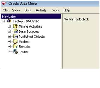

The Navigator

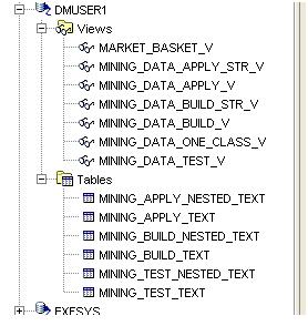
Before commencing any data mining exercise you will want to explore your data. To do this you will need to expand the Data Sources branch of the tree in the Navigator pane.
When expanded you will get a list of all users in the database who has some data visible to you or publicly to all users in the database. You only need to look for your Oracle Data Miner user. This will be the one you created as part of the installation steps given previously. By clicking on your ODM user you will see the branch will divided into Views and Tables. By expanding these branches you will be able to see what views and tables have been defined in your ODM user. The tables and views that you will see will be those that were defined as part of the installing steps given previously.

Loading/Importing Data

There are a number of ways of getting data into your ODM schema. As your ODM schema is like any other oracle schema you can use all the techniques you know to copy and load data into the schema. The ODM tool on the other hand has a data Import option, which can be found under the Data menu option. ODM uses SQL*Loader as the tool to load data into your ODM schema.
Before you select the Import option you will need to set the location of the SQL*Load executable. To do this, select Preferences from the Tool menu (Tool -> Preferences). In the Environment tab enter the location or browse for the executable.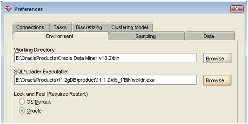
When you have specified the location of SQL*Loader you can now load CSV type files into you ODM schema. Select the Import option from the Data menu. This will open the File Import Wizard. After the introduction screen you can enter the name of a text file or search for the file.

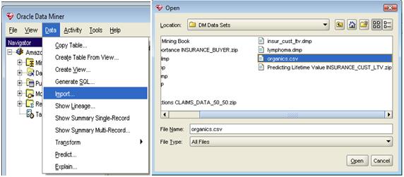
In the example given here we will load a file of transactions from a grocery retailer for organic purchases.
On the next screen of wizard you can specify what the delimiter is, state if the first record contains the field headers. The Advanced Setting button allows you to enter some of the SQL*Loader specific setting, like skip count, max errors, etc.

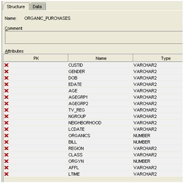
The next screen of the wizard allows you to view the imported fields that were in the first row of the organics.csv file. You may need to do some tidying up of the column names, change the data types and the sizes for each attribute.
The next screen of the wizard allows you to specify the name of the table that the data should be inserted into. If a new table is needed then you can give the table name. If the data is to be appended to the data of an existing table then that table can be select from the drop down list. In our example you will need to select that the data will go into a new table and give the name of the new table name, e.g. ORGANIC_PURCHASES. At this point you have entered all the details and you can proceed to the last screen of the wizard and select the Finish button. It will take a minutes or so for the data to be loaded. Once the data is loaded the table will appear in the Navigator pane under Tables and the table structure will appear in the main part of the ODM window. You can now select the Data tab to look at the data that has been loaded.

Exploring Data

Before beginning any data mining task we need to performs some data investigation. This will allow us to explore the data and to gain a better understanding of the data values. We can discover a lot by doing this can it can help us to identify areas for improvement in the source applications, as well as identifying data that does not contribute to our business problem (this is called feature reduction), and it can allow us to identify data that needs reformatting into a number of additional features (feature creation). A simple example of this is a date of birth field provides no real value, but by creating a number of additional attributes (features) we can now use the date of birth field to determine what age group they fit into.
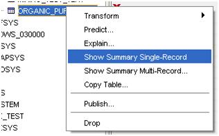
To begin exploring the data in ODM, we need to select the table or view from the navigation tree. Hole the mouse over the table/view name and right click. From the menu that now displays, select the Show Summary Single-Record. We will come back to the other menu options when we cover the next topic, Data Transformations.

The Data Summarization screen will present some high level information for your data. Taking our Organics data we can explore the ranges of values for each attribute. There is a default setting of 10, which is the number of divisions that ODM will divide the data into. During the data exploration exercise you may want to vary this value from 5 to 20 to see if there are any groupings or trends in the data. This value can be changed by pressing the Select All button followed by the Preferences button.
The following couple of example will illustrate how using the data exploration tool in ODM can help you discover information about your data in a simple graphical manner. The alternative is to log into SQL*Plus or Oracle Developer to write and execute queries to do something similar.
For the fist example we will select he Gender attribute. Although we have our number of bins set to 10, we only get 5 bins displayed. The tool will try to divide the data in to 10 equally spaced bins, but if insufficient data exists then it will present the histogram with the existing set of distinct value.

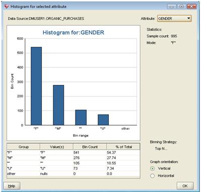
From this example on the Gender attribute we can see that there are five distinct values. F for female, M for male, U for unknown, “” (space) for records that contain a space and Other for records that contain a null. From this data we can work out that maybe we should only have three possible vales (F, M, U) but we have 105 records where we do not have a value and this equates to just over 10% of the data samples. This is a sizeable number of records. So one of the steps in the Data Transforation phase (or data clean-up) is what do we work out what to do with these records. This can include removing the data from the data set, working our what the correct value should be or changing the value to U for unknown.
For our second example we will look at the MINING_DATA_BUILD_V view (this can be found under the views branch in the navigator pane). Again right click on this object and select Show Summary Single-Record to bring up the Data Summarisation window. One of the first things that you will notice is that we get a lot more details relating to each attribute.

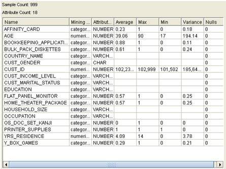
Some of these extra details include the average, max, min variance and the number of null values. Again we can go exploring the data, changing the number of bins to varying sizes to see if there is any hidden information in the data. An example of this is if we select AGE and set the number of bins to 10. We get a nice histogram showing that most of our customers are in the 31 to 46 age ranges. So maybe we should be concentrating on these.

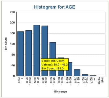
Now if we change the number of bins to 30 can get a completely different picture of what is going on in the data. Now we can see that there are a number of important age groups what stand out more than others. If we look at the 21 to 34 age range, in the first histogram we can see that there is not much change between each of the age bins. But when we look at the second histogram for the 30 bins for the same 21 to 34 age range we get a very different view of the data. In this second histogram we see that that the ages of the customers vary a lot. What does mean. Well it can mean lots of different things and it all depends on the business scenario. In our example we are looking at an electronic goods store. What we can deduce from this second histogram is that there are a small number of customers up to about age 21. Then there is a big jump. Is this due to people having obtained their main job after school having some disposable income. This peak is followed by a drop off in customers followed by another peak, drop off, peak, drop off etc. Maybe we can build a profile of our customer based on their age just like what our financial organisations due to determine what products to sell to use based on our age and life stage.

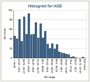
From this histogram we can maybe categorise the customers into the follow
• Early 20s – out of education, fist job, disposable income
• Late 20s to early 30s – settling down, own home
• Late 30s – maybe kids, so have less disposable income
• 40s – maybe people are trading up and need new equipment. Or maybe the kids have now turned into teenagers and are encouraging their parents to buy up todate equipment.
• Late 50s – These could be empty nesters where their children have left home, maybe setting up home by themselves and their parents are building things for their home. Or maybe the parents are treating themselves with new equipment as they have more disposable income
• 60s + – parents and grand-parents buying equipment for their children and grand-children. Or maybe we have very techie people who have just retired
• 70+ – we have a drop off here.
As you can see we can discover a lot in the day by changing the number of bins and examining the data. The important part of this examination is trying to relate what you are seeing from the graphical representation of the data on the screen, back to the type of business we are examining. A lot can be discovered but you will have to spend some time looking for it.
In my next posting, I will cover some of the Data Transformation function that are available in Oracle Data Miner.
Brendan Tierney