Introduction

In this blog post we will load a large dataset into Snowflake and then evaluate the performance of joins in Snowflake.

Loading large data into Snowflake

Dataset

The dataset we will load is hosted on Kaggle and contains Checkouts of Seattle library from 2006 until 2017. You can also download the data and see some samples here.
The dataset consists of two main file types: Checkouts and the Library Connection Inventory.
To start off the process we will create tables on Snowflake for those two files.
The DDL statements are:

A detail to notice is that the book contained in each checkout event can be linked to the table containing inventory of books using the BibNumber .

Loading the dataset into Snowflake

To load the dataset from our local machine into Snowflake, we will use SnowSQL – a command line application developed by Snowflake for loading data. SnowSQL is currently the only way to upload data from a local machine into Snowflake’s staging area.
SnowSQL can be used to fully automate the loading procedure. It does authentication of users and the command line interface is one the best we’ve seen mainly because of excellent autocompletion support.
The process will be as follows:

1. Use the PUT command to upload the file(s) into Snowflake staging area
2. Use the COPY INTO command to populate tables we defined with data in Snowflake staging area

Uploading files to Snowflake staging area

Once we download the data from Kaggle (2GB compressed, 6GB uncompressed), we can start with the uploading process.
First we will define a stage (staging area) on Snowflake. During the definition of a stage, it’s usually also good to specify the default file format.
Our data is in CSV format with commas (‘,’) being the field delimiter. The columns containing string values in the Inventory file have quotes around them so we will add another parameter to handle this. The file format can be defined as follows:

Now we can define the stage:

Copying the data from local machine into the stage doesn’t require much validation. The file format is not checked during the execution of PUT command but only during the COPY INTO command.Now we can define the stage:
To copy the files we will use following statements that also utilize Regular Expressions:

In this case compressed file that get uploaded to Snowflake are of average size ~200MB. Ideally we would split this into even smaller files of sizes 10-100MB so that the COPY INTO command can be better parallelized. You can read more about these considerations in Snowflake’s manual.

Copying the data into tables

The process of copying the data into tables is usually more complicated and really depends on the quality of your data.
Now we are going to copy the staged files into according tables on Snowflake.
We can then copy the data as following:

We used the ON_ERROR clause because some rows from 2005 and 2006 missed the date column. You could also ignore those errors but we decided to remove those which didn’t have values. Loading the “Library_Collection_Inventory.csv” file was slightly more difficult as the string columns were enclosed with double quotes. This was dealt with in the definition of the file format. Another issue is that some string columns have extreme lengths (1000+ characters) so we decided to truncate those values ie. discard them. We added an extra TRUNCATECOLUMNS clause to deal with this.
The statement we used is the following:

Before doing the actual loading it’s a good practice to run the COPY INTO statement in validation mode by adding the VALIDATION_MODE clause. In validation mode Snowflake will not load the rows to the corresponding table but rather it will parse the data (according to the schema of your table) and return all the rows that were successfully parsed. It’s a great way to validate the quality of your data before actually loading it.

Joins on large tables

Now that we managed to load all the files into Snowflake let’s check the size of our table containing checkouts:

The query returned 91 931494. So we have almost 92 million rows.
Now we are going to test how Snowflake handles a join between two large transaction tables with 90M rows each. The tests will be done on the smallest XS instance.
We will join the checkouts table with itself on two fields: CheckoutDateTime and ItemBarcode.

Attempt 1

We will join the table with itself and see how the data is loaded. Specifically is the data loaded from the remote storage or the cache:

We started the query with clean caches ie. data wasn’t loaded into the local machine cache.
The resulting execution plan was:

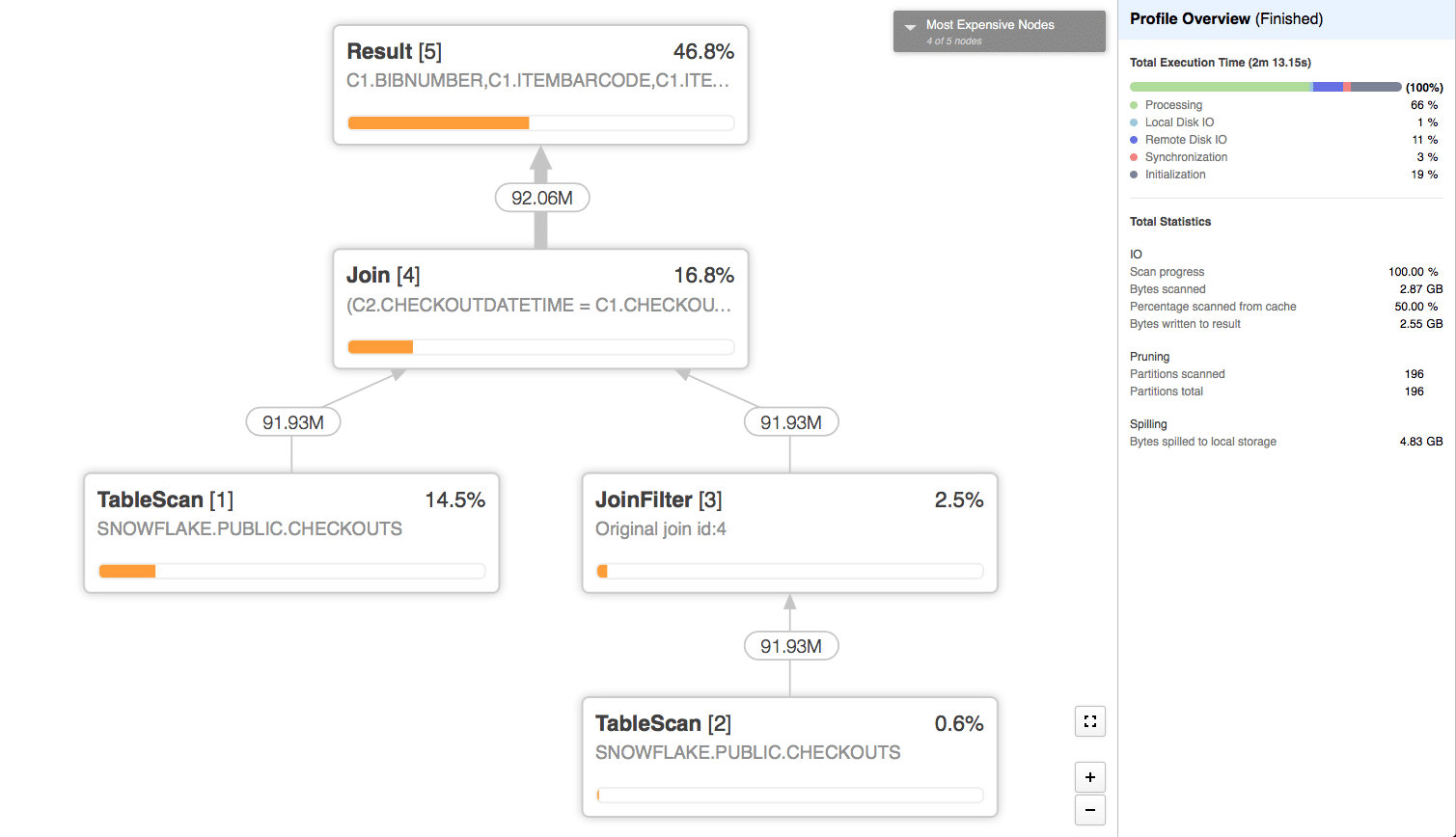
The TableScan[1] operator which took 14.5% of the time actually loaded the data exclusively from remote storage while the TableScan[2] operator loaded it from the cache.
The most time consuming operation in the query was the Result operator which wrote the Result Set into Snowflake’s proprietary Key-Value store.
The join operator was the second most time consuming operator because it spilled to disk 4.83GB of data (compared to the output of 2.55GB).

Attempt 2

We will now create a clone of the checkouts table and then join it with the original table.

Now let’s join them:

The resulting execution plan is:

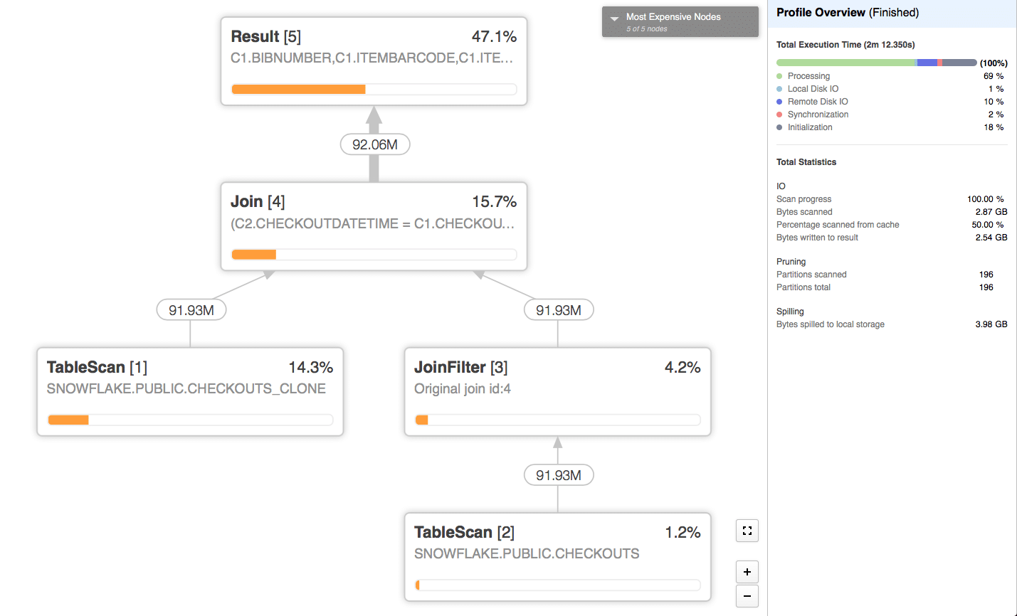
We can see that again only half of the data was loaded from remote storage and the other half was loaded from the cache. We assume that this happens because the join operator for one side first loads the data from remote storage into the local machine and then because cloned tables share the same underlying partitions, the optimizer can use the cached data for the join operator on the other side.
Again the same reasons made the Result and Join operators take the same amount of time.

Attempt 3

Now we will try to create an actual copy of the table using the CREATE TABLE AS statement:

The query is again:

The execution plan is:

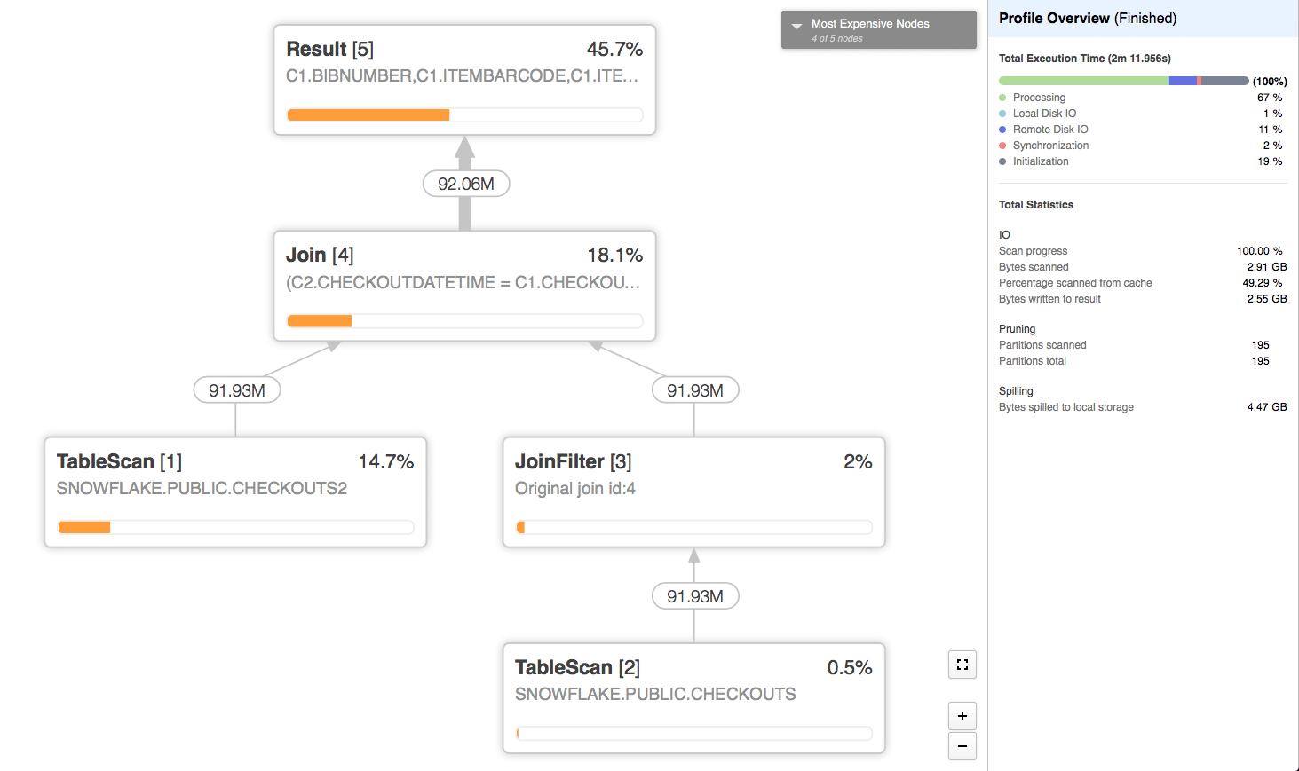
This time data was fully loaded from the remote storage for both TableScan operators.
But it’s important to notice that this didn’t affect the overall execution time of the query that much – 132 seconds compared to 132 and 133 seconds for the first two attempts.
Because we saw the issues with Join operator spilling data to disk, it is a good idea to try a larger Virtual Warehouse size.

Increasing the size of our Virtual Warehouse

As we used the XS virtual warehouse before, now we will try the S sized one. The XS sized warehouse utilizes a single (1) server per cluster (we use only a single cluster). For the usage it bills 1 credit per hour. The S sized instance utilizes two (2) servers per cluster and is billed as 2 credits per hour.
We will keep the same query from Attempt 3.
The resulting execution plan is:

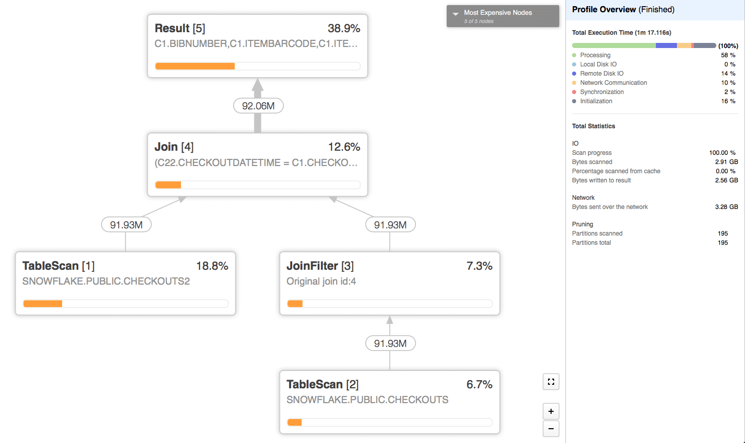
We can see that this time the query finished much faster 77 seconds compared to 132 seconds. This is mainly due to the fact that the Join operator didn’t have to spill anything to disk. This is due to the fact that larger Virtual Warehouses get more memory so the join could have been completed in-memory.

Enjoyed this post? Have a look at the other posts on our blog.
Contact us for Snowflake professional services.
We created the content in partnership with Snowflake.