Databricks JSON Guide – Read, Parse, Query & Flatten Data

JSON and Databricks should work smoothly together. They don’t.

Yes, Databricks can parse simple JSON files. It can also partially infer their schemas and process them in large chunks.

But converting JSON into clean, query-ready tables that are easily maintainable down the road? This is where things start to crack.

Try to start up your JSON to Databricks pipeline, and the pain points show up almost immediately:

1. JSON inputs arrive with deeply nested arrays that must be carefully flattened or normalised before they’re usable,
2. Real-world feeds introduce inconsistent fields, shifting data types, and partial records that trigger schema drift or schema-inference failures, and,
3. As schema complexity or data volumes grow, Databricks’ parsing and inference stages can become a performance bottleneck or even exhaust driver memory.

This guide cuts through all this mess.

You’ll learn how JSON behaves in Databricks, how to reshape it safely, how to build a stable model on Delta, and where automation saves you days of manual work.

TL;DR for the data engineer in a hurry:

• You’ll learn how JSON actually behaves inside Databricks, from the moment it lands in storage to the point it becomes a clean Delta table.
• We’ll cover ingestion patterns (batch files and Auto Loader streaming), the three ways Databricks can store JSON (raw strings, strict structs, and VARIANT), and how to choose the right one.
• You’ll see how to manage schemas manually, where Databricks helps, and how automated schema generation removes the pain entirely.
• Then we’ll dig into extracting fields with manual approaches (SQL and PySpark), flattening nested structures in the Silver layer, and handling arrays, hierarchies, and nulls without breaking your logic.
• I’ll show you several caveats of manual pipelines and how they can easily collapse under pressure.
• Finally, how to keep everything stable at scale with an automated solution.

JSON to Databricks Fundamentals

Before we go any further, I need to make sure you understand the basics.

If you’re already acquainted with the basics, go ahead and move on to ingesting or storing JSON in Databricks.

If you’re still here, then your core challenge is simple: You have to turn raw (and often unpredictable) JSON into relational tables in Databricks, but don’t know where to get started.

This section sets the stage so the rest of the blog post actually makes sense.

The big picture

Before we start pulling JSON apart, I need to show you where it actually fits inside the Databricks Lakehouse.

Databricks treats JSON as one of those formats you can dump in quickly and worry about later. That sounds great, until you realise “later” usually becomes your problem.

In the Lakehouse model, you and I don’t get to skip steps. JSON arrives raw, messy, and full of surprises.

Databricks can store it, stream it, and infer just enough structure to keep things moving, but it won’t magically convert it into clean tables. That’s still on us.

The Medallion Architecture Map

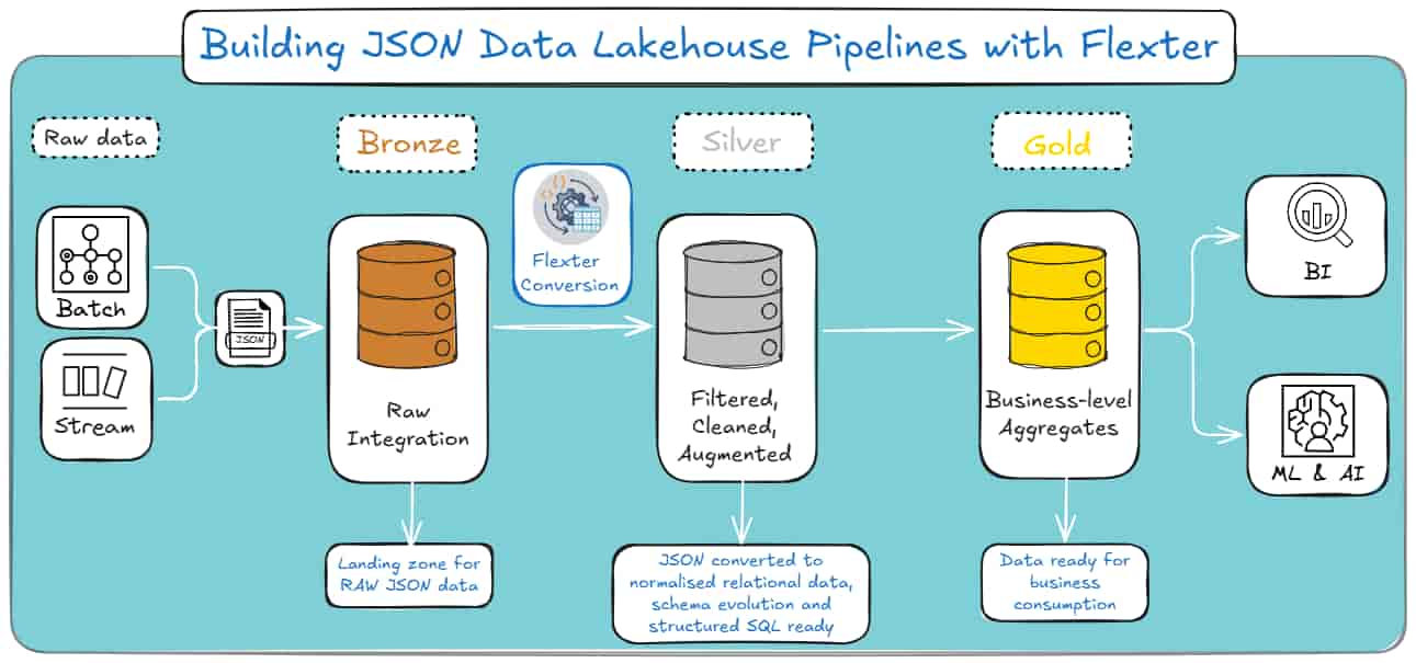
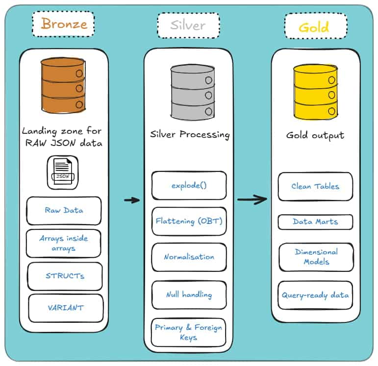
That’s where the Medallion Architecture comes in: it’s the path your JSON takes through the Lakehouse.

Databricks doesn’t magically turn raw JSON into clean tables; you and I have to push it through each layer with purpose.

Bronze Layer (Raw): This is where everything lands. Raw strings, VARIANT, unflattened Structs; whatever the source throws at you.

The goal here isn’t beauty. It’s simply getting the data in, intact, and ready for the next step.

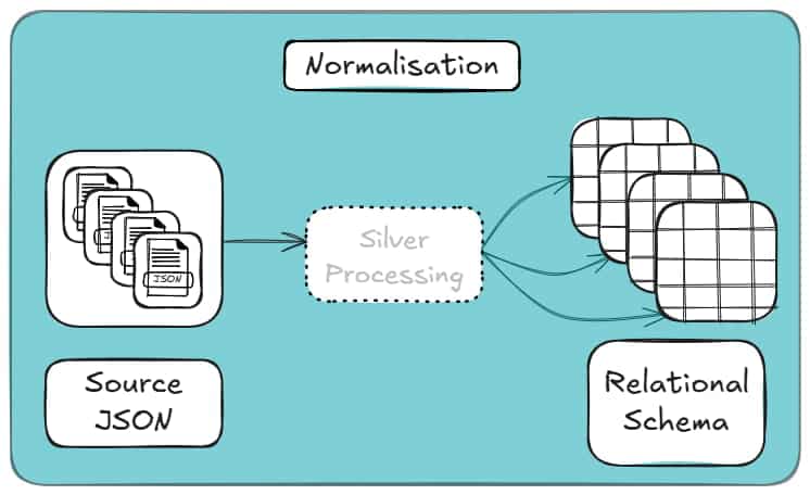
Silver Layer (Cleansed & Conformed): This is where the real work begins. You flatten the structures, explode the arrays, and normalise the mess into something that finally resembles relational tables.

This is the layer where your JSON stops behaving like a wild document and starts acting like data you can trust.

Gold Layer (Curated): Once the Silver layer is stable, you aggregate it into star schemas, data marts, and reporting views.

This is the “don’t break anything the business depends on” layer. Clean, predictable, and built for analytics.

Each layer builds on the last. Skip one, and everything downstream becomes a headache.

And here’s how the Medallion architecture looks if you’re a visual learner:

The Challenge: The Silver Layer

Here’s the real problem: you start with raw JSON that’s happily nested six layers deep, and you’re expected to turn it into clean, relational tables that behave as they came from a well-designed database.

JSON doesn’t care about your model, your joins, or your sanity. It just dumps whatever structure it wants into your lap during the Bronze Layer. And that’s OK.

But the next part is an unavoidable hell. You have to pull hierarchical data apart, flatten it or normalise it, and make it fit into something SQL can actually work with.

And Databricks won’t do this for you. It gives you the tools, sure, but you’re the one who has to wrestle the structure into shape.

This is the challenge we’re dealing with: the Silver Layer, where you will take semi-structured chaos and turn it into something consistent, predictable, and ready for analytics in Gold.

Let’s dive deeper and see each layer one by one.

Storing and Typing JSON in Delta: Strings, Structs, and VARIANT

When you bring JSON into Delta Lake, you need to decide how much structure to apply and when.

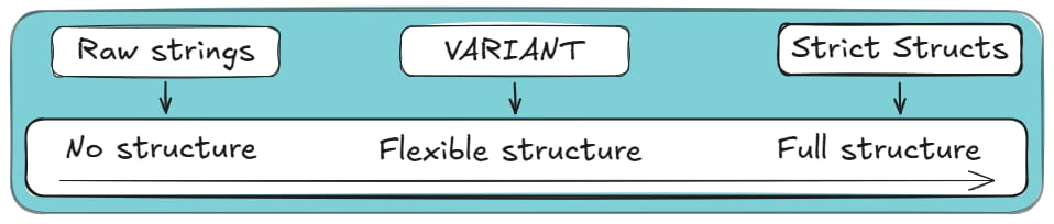
Delta gives you three broad storage patterns: keep JSON as raw text (i.e. raw strings), parse it into strict structs, or store it inside the more flexible VARIANT type.

Each approach comes with different trade-offs around performance, schema evolution, storage efficiency, and pipeline maintenance.

However, the main difference among the three methods is the level of structure enforced at ingestion. Here’s how it looks in a left-to-right diagram:

Below, I’ll walk you through each option, explain how Databricks handles them under the hood.

Option 1: Raw Strings (The “Safe” Way)

Storing JSON as plain strings is the most robust and schema-agnostic approach.

Instead of parsing the data at ingestion time, you write each JSON document into a STRING column exactly as it arrives.

This keeps your pipeline resilient to structural drift, irregular fields, or unexpected nesting.

Databricks doesn’t attempt to infer or validate JSON structure when you store it as a string, so ingestion is fast and stable even with inconsistent payloads.

Downstream, you can parse the JSON on read using functions like from_json, get_json_object, or SQL/JSON path expressions.

This model is especially useful when the schema changes frequently or when you need to archive raw data for compliance or replay purposes.

The downside? Everything becomes schema on read.

 How can you create a column to store JSON as Raw Text?

You can use the following SQL snippet:

Note: Because the JSON is stored as raw text, fields must be parsed at query time, which adds CPU overhead.

When to use Raw Strings to store JSON in Databricks?

With Raw Strings and a Schema on Read approach, querying requires explicit parsing, and performance depends on repeatedly extracting fields from text.

If your users rely on SQL for analytics, this quickly becomes cumbersome, and repeated parsing can slow down queries on large datasets.

Use raw strings when you want maximum safety and minimal ingestion friction, but not for workloads where the JSON structure is well understood or heavily queried.

Option 2: Strict Structs (The “Traditional” Way)

The strict struct model parses JSON into a well-defined schema at ingestion time.

Databricks leverages Spark’s schema inference, or user-provided schemas, to convert JSON into structured STRUCT, ARRAY, and primitive types.

This gives you strong typing, stable columns, and fast relational-style querying once the data lands in Delta.

Using Strict Structs is closer to what people call a schema on write approach.

When to use Strict Structs for storing JSON in Databricks?

The main benefit of struct-based storage is performance.

Because JSON is parsed once and stored in Delta Lake’s columnar format, queries avoid repeated JSON parsing and can benefit from predicate pushdown, column pruning, and Delta’s metadata optimisations.

For workloads that depend on reliable querying, this approach is more suitable than the other options I’ve included in this section.

How would you use Strict Structs to load your JSON into Databricks?

Here’s an SQL snippet that creates a struct, loads JSON data into it and then queries it.

Unlike the raw STRING approach, the JSON is parsed once at ingestion and stored as typed, nested columns in Delta.

At query time, Databricks can apply column pruning and predicate pushdown without repeatedly parsing JSON.

There are several downsides to strict structs. The first is schema rigidity.

Any structural change in the incoming JSON, a missing field, a new nested object, or a field that changes type between batches can break the pipeline or cause partial ingestion.

Schema evolution features help, but they don’t handle every edge case, especially when deeply nested arrays or inconsistent types appear.

The latter case will cause a type coercion failure, which occurs when a conflicting field is present, not when new fields are added to the schema.

For example, let’s consider two Batches, where:

• Batch 1: arrives with “user_id”: 1005 (Integer), and
• Batch 2: arrives with “user_id”: “1005A” (String).

If you use a strict struct model, Batch 2 will fail hard.

This is because Databricks cannot fit the string “1005A” into the integer column created by Batch 1.

This usually results in the entire batch failing or in rows being quarantined in a “dead letter queue”, requiring manual intervention to resolve.

The verdict?

Struct-based typing works best when the source JSON is stable or governed.

Choose strict structs when you have predictable schemas, strong SLAs, and SQL-heavy consumers, but be prepared to manage schema drift carefully.

Option 3: VARIANT (The “Modern” Way)

Delta’s VARIANT type provides a middle ground between raw strings and strict structs.

A VARIANT column stores semi-structured data in a parsed, binary-encoded form that still preserves the hierarchical JSON structure.

Unlike raw strings, the data is stored semantically; unlike strict structs, it doesn’t require a fixed schema.

How “Shredding” Makes VARIANT Fast

At this point, a reasonable question comes up: if VARIANT is this flexible, shouldn’t it be painfully slow to query?

Normally, yes. Reading semi-structured blobs at scale tends to end badly.

This is where Databricks uses a technique called shredding (conceptually similar to Snowflake’s sub-columnarisation).

When you write JSON into a VARIANT column, Databricks doesn’t just store it as one opaque object.

The engine analyses the JSON structure and identifies frequently accessed paths such as event_type or user.id.

Those paths are then extracted and stored internally as dedicated, hidden columns inside the underlying Parquet files.

The practical effect is that queries targeting common fields don’t need to scan or parse the entire JSON payload.

They can skip irrelevant data and read only the relevant shredded columns.

You get much closer to STRUCT-like performance for frequently accessed paths, while keeping the flexibility of VARIANT and avoiding early schema enforcement.

When to use VARIANT to store your JSON in Databricks?

VARIANT is particularly useful for datasets where fields appear inconsistently, arrays vary in shape, or new properties surface over time.

Databricks can index and scan VARIANT data more efficiently than raw strings, and querying is more ergonomic: SQL functions can navigate nested structures without reparsing the original JSON text.

VARIANT reduces the risk of ingestion failures due to schema evolution, while still offering performant read access compared to storing JSON as text.

How to create a table with a VARIANT column?

Here’s an SQL code example that uses VARIANT columns inside Delta in order to load and query a JSON payload.

Compared to storing JSON as a STRING, VARIANT avoids repeated text parsing and benefits from internal shredding, resulting in far better query performance.

Compared to Strict Structs, VARIANT does not enforce a fixed schema at ingestion, making it more resilient to schema evolution.

The trade-off is that queries still require path expressions, and very heavy or deeply nested VARIANT structures may not perform as well as fully flattened or normalised relational models.

Additionally, VARIANT does not automatically normalise nested arrays into exploded tables, so analysts may need to project or flatten fields manually when performing relational analytics.

Use VARIANT when your schema changes frequently, but you still need fast analytical querying without enforcing a rigid structure at ingestion time.

Decision Matrix to Help you Decide Between the three Storage Methods

To sum up all of this information, here’s a comparison table for the three JSON to Databricks storage methods:

Dimension	Raw Strings	Strict Structs	VARIANT
How it stores data	JSON kept as plain text (blob).	JSON parsed into fixed columns.	Binary-encoded; frequent paths are “shredded” into columns.
Ingestion reliability	Very high. Ignores content.	Fragile. Breaks heavily on type mismatches (e.g. “id”: 100 vs “100A”).	High. Adapts to new fields automatically.
Query performance	Slow. No data skipping; requires full table scans.	Fastest. Native columnar read.	Close to STRUCT-level performance for frequently accessed paths, though STRUCT columns remain faster and more predictable overall.
Storage Cost	High. Text compresses poorly compared to binary.	Low. Efficient encoding.	Low. Comparable to structs.
When to avoid	When you care about storage costs or query latency.	When upstream data types are messy or unstable.	When you need strict constraints (e.g. NOT NULL) on nested fields.

If this table has a lot of information for you, here’s the “meat”:

• Use VARIANT when your JSON changes shape often, and you need reliable ingestion with flexible querying.
• Use strict structs when the schema is stable, and downstream consumers want fast, relational access.
• Use raw strings only when you need to preserve the payload exactly as delivered, or to keep the landing zone as simple as possible.

Ingesting JSON in Databricks: Batch and Streaming (The Bronze Layer)

Now that you know all about storing JSON in Databricks, let’s talk about ingesting JSON into Databricks.

It is also known as the part of the pipeline where everything should be boring, but somehow never is.

JSON shows up in folders when it feels like it, sometimes late, sometimes twice, sometimes with extra fields it forgot to mention.

Databricks gives you three main ways to deal with this in the Bronze layer: traditional batch ingestion, streaming ingestion with AutoLoader, and AutoLoader-based batch-like ingestion.

Want a TL;DR? Both work. Both can also hurt you if used in the wrong place.

Read the full section to find what suits you best, or skip to the final comparison section.

(For this section on loading methods, I assume that you chose VARIANT columns as your storage option.)

File-base JSON Batch Ingestion to Databricks

Classic batch ingestion is the approach everyone starts with.

You point Databricks at a folder of JSON files, read them, do a bit of light transformation if needed, and write the result to Delta.

Here’s a minimal Python example for implementing that batch-loading job, using the PySpark library:

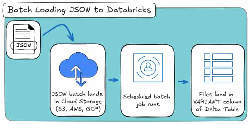
The batch loading job scans the directory you specify, lists all matching JSON files, reads them once, and stops.

If you rerun the job with the same input path, Spark will happily reread the same files and overwrite the output.

And most importantly: Spark does not remember anything about previous runs.

Here’s how it looks as a high-level process:

This approach works well when:

• You have a static or bounded dataset,
• You’re doing a one-off import or backfill,
• The folder structure itself encodes incrementality (for example, one folder per day).

The problem is that incrementality is entirely your responsibility.

If new files arrive late, arrive twice, or land in the wrong folder, Spark will not help you. You have to manage:

• Which paths are read per run,
• How to avoid re-reading old files,
• What happens if a job partially fails.

For small or controlled datasets, this is fine. For anything resembling a real feed, this is where batch ingestion starts to creak.

Auto Loader for Batch and Streaming Ingestion

Auto Loader exists because incremental file ingestion kept being re-implemented by hand, and almost always badly.

Someone would scan a folder, remember which files they think they processed, rerun the job, and then spend the next week explaining why numbers doubled.

Auto Loader fixes that class of problem by treating files as a stream, even when you don’t actually want a continuously running streaming job.

That distinction matters more than the name suggests.

Under the hood, Auto Loader tracks files, persists state, and handles incremental discovery at scale. What you choose is how you run it.

Autoloader for Loading your JSON to Databricks (Streaming Mode)

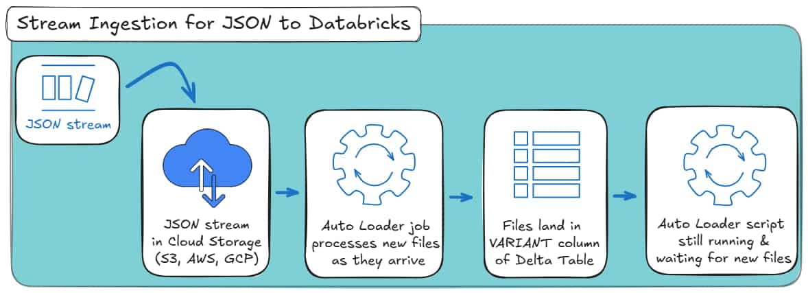
This is Auto Loader in its original, intended form: continuous ingestion.

New JSON files arrive in cloud storage, Auto Loader detects them, parses them, and appends them to the VARIANT column of a Delta table as they appear.

The job keeps running and reacts to new data instead of being restarted on a schedule.

A minimal streaming setup looks like this:

What’s happening here:

• cloudFiles activates Auto Loader.
• cloudFiles.format = json tells it how to parse incoming files.
• schemaLocation stores inferred schemas and schema evolution metadata.
• The checkpoint stores progress, so Spark knows which files have already been processed.
• The job keeps running, ingesting new files as they arrive.

This mode makes sense when:

• Files arrive continuously throughout the day,
• You want near-real-time availability in the Bronze layer,
• You’re comfortable running a long-lived streaming job.

Here’s how it looks as a high-level process:

That said, most teams don’t actually need real-time ingestion. They need safe incremental ingestion. And this is where Auto Loader quietly shines.

Batch-like loading your JSON with Autoloader

You still use Auto Loader. You still get incremental file tracking, schema persistence, and fault tolerance. But the job runs once, processes everything new, and stops.

Here’s the same ingestion rewritten in batch-style mode:

Did you notice the crucial line? Search again for:

This tells Spark to:

• Process all currently available new files,
• Commit the results,
• Stop the job.

The next time you run the exact same code, Auto Loader will only ingest files that arrived since the previous successful run.

You do not change input paths. You do not track folders. You do not risk rereading old data.

Here’s how it looks as a high-level process:

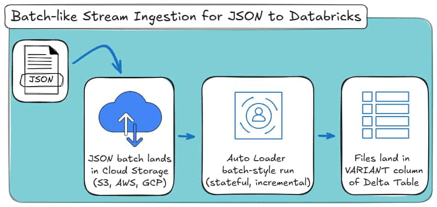
Conceptually, this behaves like a batch. Operationally, it behaves like streaming.

That combination is why Databricks generally recommends Auto Loader even for “batch” ingestion scenarios.

Batch vs. Streaming Ingestion for JSON to Databricks

At a high level, Databricks gives you three practical ingestion patterns for JSON in the Bronze layer:

1. Traditional batch ingestion,
2. Auto Loader in streaming mode,
3. Auto Loader in batch-style mode.

They all get data into Delta. The difference is how much state they carry and how fragile they become over time.

Here’s a comparison table to put it all together:

Dimension	Traditional Batch Ingestion	Auto Loader (Streaming Mode)	Auto Loader (Batch-style Mode)
Execution model	Discrete batch jobs	Continuous streaming job	Scheduled batch job
State between runs	None (stateless)	Persistent (stateful)	Persistent (stateful)
Incremental file handling	Manual (paths, partitions, logic)	Automatic	Automatic
Risk of reprocessing data	High if not carefully managed	Very low	Very low
Handling late-arriving files	Manual and error-prone	Built-in	Built-in
Schema persistence	None	Stored and evolved	Stored and evolved
Operational complexity	Low at first, grows over time	Higher (long-running jobs)	Moderate
Typical use case	One-off loads, backfills	Near-real-time ingestion	Ongoing feeds with scheduled runs
Bronze-layer suitability	Limited for real feeds	Good	Excellent

What Auto Loader Actually Solves (and What It Doesn’t)

Auto Loader helps with ingestion mechanics, not data modelling or schema management.

It does:

• Track processed files reliably,
• Prevent double ingestion,
• Handle incremental file discovery at scale,
• Persist schema information across runs.

Sadly, it does not:

• Flatten nested JSON (for deeply nested or complex JSON files),
• Normalise arrays,
• Fix inconsistent payloads,
• Design or enforce a relational schema.

All of these problems actually belong in the Silver layer.

That’s why you need to read up on my next section on manual vs. automated JSON schema generation in Databricks.

JSON Databricks features for Defining and Managing Schemas

At this point, your JSON is safely landing in Delta. Great. That was the easy part.

Now comes the uncomfortable question Databricks quietly hands back to you:

And more importantly:

If you were hoping Databricks would magically convert your JSON into clean, relational tables, this is where reality sets in.

Databricks is good at ingesting JSON.

It is far less opinionated about what the schema should be, and completely agnostic about relational modelling.

That gap is where most pipelines start to rot.

Why Schema Definition is the real bottleneck

Schema decisions in Databricks are not cosmetic. They determine:

• Whether your pipeline survives schema drift or collapses at 2 a.m.
• Whether analysts can query data directly or need PySpark babysitting.
• Whether Silver-layer logic is stable, or rewritten every sprint.

Databricks provides multiple ways to infer or define schemas, but they are often treated as interchangeable. They are not.

Each approach comes with sharp trade-offs that only show up once your JSON stops behaving nicely.

Before we discuss automation, we need to be honest about what the manual path actually looks like.

The manual approach: what Databricks really infers

Let me show you two manual coding approaches for schema inference in the JSON to Databricks challenge.

Example JSON input (realistic, not toy-perfect)

Assume your source delivers JSON events like this:

File 1:

File 2:

File 3:

Method 1: schema_of_json (precise, local, misleading)

schema_of_json answers exactly one question:

Nothing more than that. Here’s how you may use it:

The result:

That schema is correct for that one document.

Now watch how you can naïvely apply it to a dataset:

Then Databricks would:

• Pick one row,
• Infer the schema from that row,
• Ignore the rest of the data completely.

If the first row doesn’t include age, then age does not exist as far as Spark is concerned.

At this point, many engineers look for a way to “merge” schemas across rows manually.

In Databricks and Spark SQL, there is no safe or supported way to do this using the schema_of_json function.

The function operates on a single JSON value. It cannot infer a dataset-wide schema, and attempting to aggregate JSON values into the driver to force a merge is both unsafe and unsupported.

This looks better. It’s also:

• Limited to a single JSON value,
• Blind to the rest of the dataset,
• Unsafe to scale beyond toy examples.

There is no schema evolution. No safety net. This is schema inference by optimism.

Method 2: spark.read.json with inferred schema (probabilistic)

Now let Spark infer the schema across files:

The result you will most likely receive:

Why is age a STRING?

Because Databricks saw:

• 30 (numeric),
• “unknown” (string).

Databricks widened the type to avoid failure. This is not wrong. It is also not deterministic.

Which means that if you change:

• File order,
• Sampling ratio,
• Partitioning.

.. and you may get a different schema tomorrow. Not stressful at all right?

This is why inferred schemas are convenient for exploration, but dangerous for pipelines you expect to trust.

Auto Loader for schema management, not schema design

Auto Loader improves the situation operationally.

It persists the schema state and evolves it incrementally:

How evolution actually works:

Let’s assume Day 1 input:

Stored schema:

But then on Day 10, the JSON input may change to this:

Auto Loader:

• Detects age,
• Adds it as a nullable column,
• Preserves existing data.

This is something neither schema_of_json nor read.json can do reliably.

But here’s the limitation: Auto Loader still performs a literal translation of the JSON tree.

Why Silver is mandatory, even with Auto Loader

Consider the following JSON:

Auto Loader produces one table:

Query result:

order_id	customer	items
101	{“name”:”Alice”,”address”:{“city”:”Dublin”}}	[{“product_id”:1,”qty”:2},{“product_id”:5,”qty”:1}]

This is schema inference working exactly as designed. But at the same time, it is also completely unusable for relational analytics.

To make this useful, you must now:

• Explode arrays,
• Split parent and child entities,
• Generate keys,
• Maintain joins,
• Rewrite everything when the structure changes.

This is the Silver-layer tax. Auto Loader merely moves it downstream rather than eliminating it.

What do you need to add to your Auto Loader approach (what the code really looks like)

To extract order items, you write:

Now repeat this:

• For every array,
• For every nesting level,
• For every schema change.

This is not hard once. It is exhausting forever.

Flexter schema generation: same data, different outcome

Flexter looks at the same JSON and answers different questions.

Instead of:

It asks:

This difference in intent is everything. Flexter does not treat schema inference as a parsing problem.

From the example above, Flexter generates:

• Orders,
• Customers,
• Order_Items.

With:

• Primary keys,
• Foreign keys,
• Stable column types
• No manual Databricks explode JSON logic.

And it stores the mapping in a metadata catalogue, so the logic is reused across files and runs.

No recursive Spark code. No fragile inference. No Silver-layer rewire every time the feed twitches.

How does Flexter achieve smart and efficient schema inference, you ask?

1. Naive mapping vs. optimised schema design

Databricks applies a literal, 1:1 mapping between the JSON tree and the target schema. If your JSON path is:

Databricks faithfully reproduces that hierarchy using nested STRUCTs and ARRAYs, leaving you to clean it up later.

Flexter doesn’t do that. Instead, it analyses and optimises:

• Data distribution across records,
• Cardinality of relationships,
• Repetition and redundancy in substructures,
• Whether a branch behaves like a true entity or just an attribute group.

From there, it makes structural decisions, not just translations. Concretely:

• 1:1 relationships are flattened automatically.
• 1:N relationships are split into separate tables.
• Repeating structures become dimension-like entities instead of duplicated blobs.

The result is not a mirrored tree. It’s a deliberately simplified relational model.

2. Redundancy detection instead of blind flattening

One of the biggest hidden costs of manual Silver-layer pipelines is silent redundancy.

Auto Loader will happily ingest the same customer, user, or reference object hundreds of times as part of a One Big Table.

It does not recognise that those substructures represent a reusable entity.

Flexter explicitly looks for these patterns. If a nested object:

• Appears repeatedly across records, and
• It is logically independent of the parent record,

Flexter isolates it and automatically generates the appropriate keys. That means:

• No duplicated customer blocks,
• No manual surrogate key logic,
• No fragile hash-based joins you have to maintain later.

You get proper primary and foreign keys without writing a line of Spark code.

3. The metadata catalog: where the “memory” lives

Another fundamental difference is where schema intelligence is stored.

Databricks persists schemas in the Delta log as a physical description of columns. It knows what exists, but not why it exists.

Flexter uses a dedicated metadata catalog (MetaDB) that stores:

• Logical schema decisions,
• Source-to-target mappings,
• Cardinality rules,
• Transformation intent.

This has two practical consequences.

First, reusability.

Once Flexter has learned a schema, it doesn’t need to re-infer it every run. You can process millions of files with consistent results without constantly re-evaluating structure.

Second, traceability.

Because the logical mapping is explicit, you can always answer questions like:

• Where did this column come from?
• Which source element populated it?
• What happens if the source structure changes?

That level of lineage is almost impossible to reconstruct once schema logic is buried in handwritten Spark code.

Manual vs. automated JSON schema inference: the honest comparison

To put it all together in one table, here’s a comparison table for all the schema inference options:

 

Question	Manual Code (Spark and SQL)	Auto Loader (native)	Flexter (Automated)
Schema inferred once	No. Schema inferred in every run.	Schema inferred once and persisted	Yes. Includes schema evolution features.
Schema evolves safely	Manual & fragile	Yes (additive only)	Yes (controlled & optimised)
Handles type conflicts gracefully	No	No (fails & widens)	Yes
Produces relational schema (normalisation)	No	No	Yes
Avoid One Big Table (OBT)	No	No	Yes
Silver-layer custom code required	High	High	None
Breaks on complex JSON hierarchies	Eventually	Eventually	Never
Engineering effort over time	Very high	High	Low
Primary Use Case	Exploration & one-offs	Reliable ingestion	Analytics-ready pipelines

If this table is too much, here’s the takeaway:

Databricks schema inference is structural, not analytical.

It faithfully mirrors JSON. It does not interpret it.

If you choose the manual path, you are agreeing to:

• Write a normalisation engine,
• Maintain it indefinitely,
• Debug schema behaviour instead of analysing data.

Flexter exists to remove that entire class of work. If your JSON is trivial, you won’t need it. If your JSON is real, you will.

Querying and Extracting JSON in Databricks

Once your JSON has been ingested and stored in Delta, it’s tempting to think back to all the hard work that you’ve done.

The data is there, Databricks understands JSON, and SQL supports dot notation (databricks sql json).

So, querying a few nested fields should be easy from this point forward, right?

And it is.. until you do it more than once.

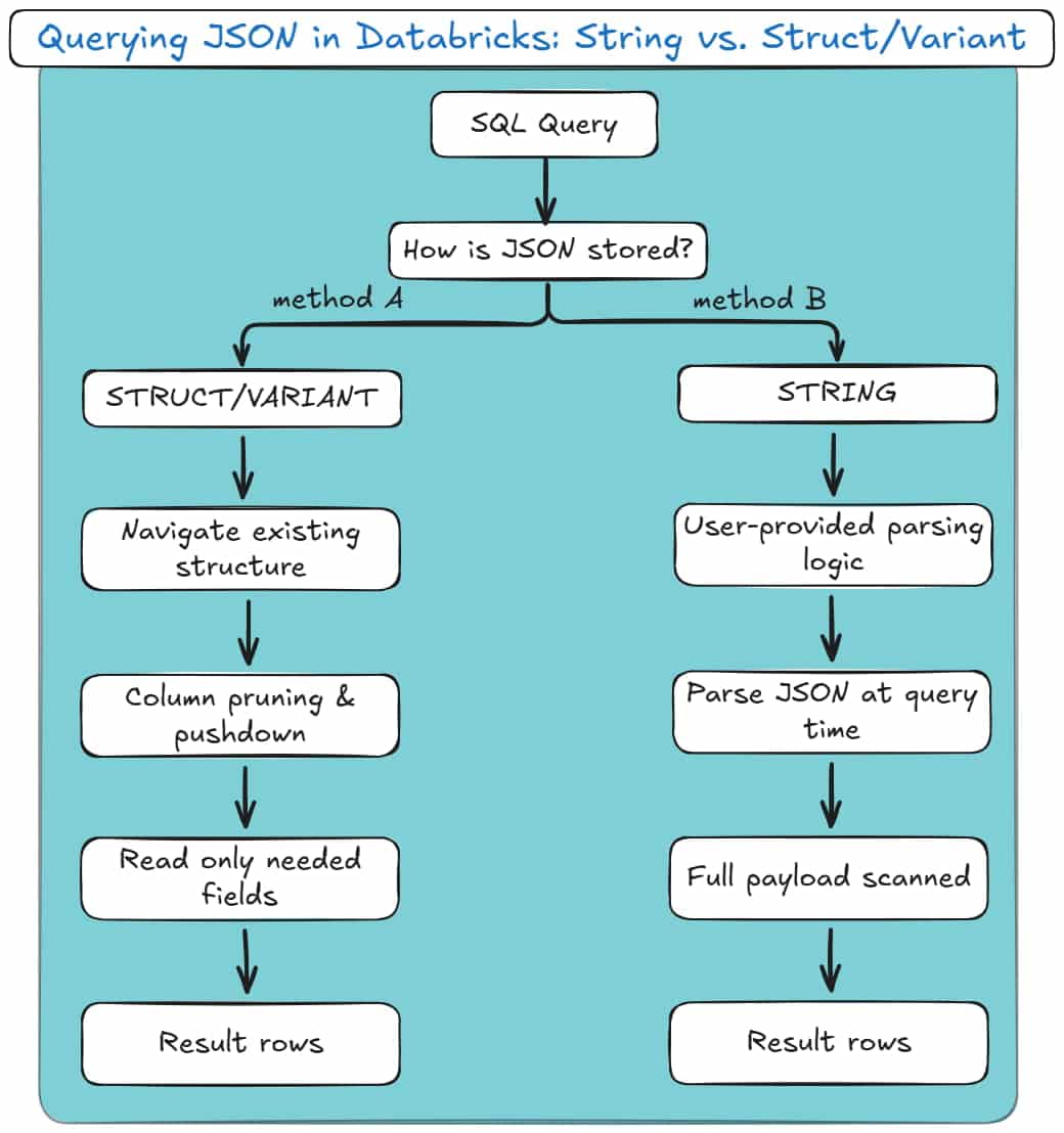
In Databricks, querying JSON is tightly coupled to how the JSON was stored in the first place.

Two queries that look almost identical can differ wildly in performance, reliability, and long-term maintainability.

The difference isn’t syntax.

It’s whether Databricks has to parse JSON at query time, or merely navigate the existing structure.

Here are your two options.

Method A: Dot Notation (Best for Structs/VARIANT)

Dot notation is the cleanest and most efficient way to extract values from JSON when the data is already structured.

This applies in two cases:

• JSON stored in STRUCT / ARRAY columns,
• JSON stored in VARIANT.

Here’s what it looks like with strict structs:

And here’s the same logical query against VARIANT:

These two queries may look similar, but the key difference lies in what doesn’t happen.

Databricks is not parsing JSON text at query time.

With strict structs, nested fields already exist as typed, columnar values in Parquet. Databricks simply reads the relevant sub-columns and ignores the rest.

With VARIANT, Databricks applies automatic shredding. Frequently accessed JSON paths are extracted into hidden, columnar representations behind the scenes.

When you query common fields, Databricks can skip most of the payload and read only the relevant paths.

In both cases, you get:

• Column pruning,
• Predicate pushdown,
• Data skipping,
• Predictable query performance.

Failures here are not query failures. They are ingestion failures.

If a strict struct breaks, it’s because the upstream JSON changed shape or type earlier in the pipeline. The query is just your messenger.

Method B: Extracting from Raw Strings

This is the fallback method, used when JSON is stored as plain text.

In this model, the JSON payload lives in a STRING column and must be parsed during query execution.

You’ll typically see one of these patterns:

Or:

Both approaches work. Both are also deceptively expensive.

In this model:

• JSON is parsed every time the query runs,
• There is no column pruning,
• There is no data skipping,
• Spark must scan the full payload for every row.

Choosing the Right Query Mechanism

Databricks gives you multiple ways to extract JSON values. They are not interchangeable.

get_json_object is string-based and always parses text.

from_json creates typed structures, but still parses on read when used against STRING columns.

Dot notation on STRUCT and VARIANT accesses pre-materialised paths and is fully optimised.

The wrong choice often looks harmless in development.

At scale, it becomes the reason dashboards slow down, clusters scale unexpectedly, and Silver-layer jobs get rewritten under pressure.

Here’s a diagram for how these two methods look:

Arrays, explode(), and the Query-Time Tax

Arrays are where JSON querying becomes expensive.

Regardless of how JSON is stored, arrays must be materialised using explode():

This expansion happens at query time. Row counts multiply dynamically, and the cost is paid repeatedly by every downstream consumer.

This is why array-heavy JSON almost always requires a Silver-layer normalisation step.

Querying exploded arrays directly works, but it doesn’t scale gracefully.

A Practical Mental Model

Querying JSON in Databricks is not about syntax. It’s about when JSON stops being JSON.

The earlier you enforce structure, the faster and more predictable queries become.

The later you enforce structure, the more resilient ingestion becomes.

Every pipeline simply shifts cost between ingestion time and query time.

Databricks gives you the tools. It does not protect you from the consequences of choosing the wrong one.

To find out how to supercharge your Silver Layer with the optimal normalisation practices, read up on my next section!

The Silver Layer: Flattening and Normalising JSON

Silver is where JSON either grows up or becomes someone else’s problem.

Here, semi-structured data is flattened, normalised, and made predictable. Arrays are exploded, hierarchies collapsed, data types are created and strictly mapped, and nulls treated as first-class concerns.

Databricks and Spark will let you avoid these decisions forever. The rest of your stack won’t even bother with such problems.

It’s up to you to choose structure now, or pay for ambiguity later.

We’ve already covered why the Silver layer is the most demanding part of the Medallion architecture.

The figure below maps the core Silver-layer concepts to their role in the overall process, showing how raw JSON is reshaped into query-ready data in Silver.

Try to keep those in mind before proceeding with the rest of this section.

Exploding JSON Arrays in Databricks

Arrays are where most JSON pipelines start to fall apart.

They look harmless in Bronze. They are not. An array in JSON usually represents a one-to-many relationship, and relational systems do not understand relationships embedded inside a single row.

In the Silver layer, arrays almost always need to be exploded.

When you explode an array, you are making an explicit modelling decision:

“One parent row produces multiple child rows.”

Here’s what that usually looks like in practice:

After this step, you no longer have “an order with items”.

You have an orders table and an order_items table. That distinction matters.

The hidden cost of delaying explode()

You can explode arrays at query time. Spark allows it. SQL allows it. BI tools will even try to do it for you.

But that cost is paid every single time someone runs a query.

Row counts multiply dynamically. Execution plans get expensive. Dashboards mysteriously slow down. Someone eventually adds more compute and calls it “scaling”.

Exploding arrays in Silver means:

• The cost is paid once.
• The structure is stable.
• Downstream consumers stop reinventing the same exploded logic.

Flattening Hierarchies

Nested structs are easier than arrays, but they still need to be handled deliberately.

JSON loves hierarchies. Analytics does not.

In Silver, flattening hierarchies usually means turning nested attributes into top-level columns.

This improves readability, simplifies queries, and allows Delta to do what it’s good at: column pruning and data skipping.

A typical flattening step looks like this:

Nothing fancy. Just explicit.

Why does this belong in Silver, not Gold

Flattening hierarchies is structural work. Gold should not be responsible for decoding JSON paths or dealing with nested field logic.

If you leave deep structs in Silver:

• Every downstream query repeats the same path expressions.
• Schema changes ripple through dashboards.
• Performance becomes unpredictable because Spark can’t optimise deeply nested access as effectively.

Silver is where you collapse the structure. Gold is where you aggregate meaning.

The One Big Table temptation

Auto Loader and schema inference encourage a “One Big Table” mindset: one row, lots of nested columns, everything technically present.

That works for exploration. It does not work long-term.

These tools make it tempting to convert JSON into a single, nested table (i.e., OBT) because it feels fast and easy.

In practice, that convenience fades as schemas evolve, complexity grows, and downstream consumers multiply. What looked simple becomes brittle and hard to change.

The more robust alternative is to normalise your source JSON, which is a process that I’ll explain in the next subsection (just keep on reading for a few more minutes).

Handling Nulls

Nulls are not a nuisance. They are information.

In JSON, nulls appear for many reasons:

• Optional fields that legitimately don’t apply.
• Fields were introduced in newer versions of the payload.
• Partial or malformed records.
• Inconsistent producer logic upstream.

Databricks will happily propagate nulls unless you intervene. In Silver, you should.

Three questions Silver must answer about nulls

• Is the field optional by design?

If yes, allow nulls and document the behaviour.

• Is the field expected to be present?

If yes, nulls represent bad data. Quarantine, default, or fail fast.

• Is the field a key or join attribute?

If yes, nulls are usually unacceptable and will break relationships downstream.

Handling this explicitly often looks like:

This is not cosmetics. This is data integrity.

The silent failure problem

The worst Silver pipelines don’t crash. They succeed quietly with worse data.

Nulls creep into keys. Joins stop matching. Aggregates undercount. Dashboards still load.

Handling nulls in Silver is how you prevent correctness issues from masquerading as performance problems later.

Normalisation versus Flattening for your Silver

By this stage, it’s easy to feel done.

The data is flat. Queries are simple. The JSON is gone. That doesn’t mean the model is right.

Flattening solves syntax, not structure.

Flattening removes nesting. It does not remove duplication, define relationships, or protect you from inconsistency.

And it often results in One Big Table (OBT) for your data, which looks like this:

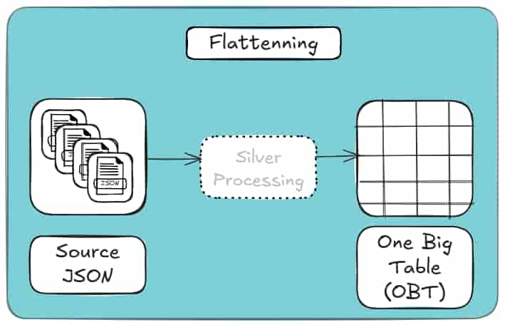
If the same entity appears repeatedly in your JSON, flattening just copies it everywhere. The table looks relational, but behaves like a document with better formatting.

Normalisation fixes that.

Normalising in Silver means separating true entities, making relationships explicit, and encoding them with stable keys. The cost is a few joins.

The benefit is correctness, reuse, and schemas that survive change. This is how it looks conceptually:

Flatten when attributes genuinely belong to a parent. Normalise when data repeats or represents its own concept.

Anything else is denormalisation pretending to be design.

For a deeper, example-driven breakdown of flattening versus normalisation, including when denormalisation makes sense, see my other blog post.

Automating the Silver Layer with Flexter

Up to this point, everything I’ve shown you has one thing in common: it works, but it’s manual.

Whether you attempt to parse your source data with Databricks JSON functions, or flatten structures with Spark, or carefully design relational schemas by hand, you’re still doing the same core tasks yourself:

• analysing nested structures,
• deciding what becomes a table vs. a column,
• handling arrays and parent-child relationships,
• keeping schemas in sync as the JSON evolves.

This is manageable for small datasets or one-off conversions.

It quickly becomes unsustainable once JSON starts changing, volumes increase, or multiple pipelines depend on the same logic.

This is where automating the Silver layer becomes not just convenient, but necessary.

The JSON Databricks Maintenance Trap

Manual Silver-layer pipelines don’t usually fail all at once. They rot.

Every explode(), every column selection, and every implicit assumption about the JSON structure become long-term maintenance obligation.

At first, this feels manageable. You add a new field. Adjust a query. Re-run the job.

Then the JSON feed evolves again.

Arrays move. Optional fields appear. A nested object becomes plural. Suddenly, logic that “worked fine for months” starts producing subtle errors instead of clean failures.

This is the maintenance trap.

Native JSON Databricks features don’t eliminate it. Auto Loader persists schema information, but it does not protect your downstream logic.

Every explode(), join, and surrogate key is still handwritten and still brittle.

Flexter removes the trap by design.

Schema logic is not scattered across notebooks. It lives in a central metadata model.

When the JSON changes, Flexter updates the model and applies those changes consistently across runs with:

• No downstream rewiring.
• No emergency patch jobs.
• No silent degradation.

Maintenance stops being reactive because the structure is no longer encoded in Spark code.

Automated JSON Parsing

Native Databricks parse JSON tools are powerful, but they all share the same assumption:

“You know what the structure should look like.”

Spark will happily parse JSON. Auto Loader will do it incrementally and at scale. But neither of them can decide how the data should be modelled. They only translate what they see.

That’s why automated ingestion still leads to manual Silver logic.

Flexter approaches parsing differently.

Instead of treating parsing as a syntactic exercise, it treats it as a modelling step.

It analyses the full dataset and determines:

• which elements behave like entities,
• which ones are attributes,
• which relationships are one-to-one or one-to-many.

Parsing and modelling happen together, not as separate phases.

The result is automation that doesn’t stop at “valid DataFrame”, but produces a usable relational structure without hand-written transformation code.

Handling JSON Complexity

Complex JSON isn’t usually just deeply nested. It’s inconsistent, as well.

This means that fields appear in some records but not others. Types drift. Arrays change shape. Edge cases show up long after the pipeline is in production.

This is where most native approaches hit their limits.

Databricks and Spark either:

• fail,
• widen types until everything becomes a string,
• or push the problem downstream to query time.

Auto Loader improves ingestion reliability, but it does not resolve semantic complexity. The burden still lands in the Silver layer.

Flexter is built for this exact scenario.

It handles:

• deeply nested hierarchies,
• Repeated substructures,
• optional and evolving fields,
• mixed cardinalities across records.

Because schema decisions are data-driven and stored explicitly, complexity does not translate into fragile code paths.

The system adapts without you having to anticipate every edge case up front.

Universal Support

One quiet limitation of manual Silver-layer pipelines is how tightly they are coupled to a specific execution environment.

Spark code written for Databricks is still Spark code. Move it elsewhere and you start rewriting. Change output targets and you duplicate logic.

Flexter deliberately decouples schema intelligence from execution.

Because modelling logic lives in metadata, not code, the same structure can be applied consistently across:

• Databricks,
• Spark,
• different storage formats,
• different downstream systems.

You’re not locking transformation logic into a notebook or a runtime. You’re defining structure once and applying it repeatedly.

That makes Silver-layer automation portable, reproducible, and far easier to reason about over time.

Automated Schema Evolution Without Pipeline Rewrites

One of the hardest parts of maintaining a Silver layer is not the initial build, but keeping it alive as the JSON evolves.

With manual pipelines, every structural change forces a reaction: new fields require code updates, renamed attributes break downstream joins, and type conflicts either fail jobs or silently widen columns.

Flexter treats schema evolution as a first-class concern.

Schema changes are detected, reconciled against the existing relational model, and applied consistently without requiring you to rewrite explode logic, joins, or key generation.

As a result, the Silver layer adapts as source data evolves, instead of becoming brittle with every upstream change.

Predictable Costs and Immediate Data Availability

Manual Silver-layer pipelines hide their true cost over time.

Engineering effort grows with every schema change, backfills become expensive, and “small fixes” accumulate into ongoing maintenance and refactoring work for you and your team.

Automating the conversion removes much of that uncertainty.

Once the modelling logic is defined, new data becomes immediately available without waiting for additional development cycles.

Schema changes no longer trigger unplanned work, and ingestion does not stall while transformations are rewritten.

This keeps projects within budget not by reducing scope, but by eliminating recurring, reactive engineering effort.

Data arrives, is shaped consistently, and is ready for downstream use without manual intervention.

Why does all of this matter?

All four of these issues exist regardless of tooling choice.

JSON Databricks features don’t cause them. Spark does not solve them.

They are intrinsic to semi-structured data, such as JSON and XML.

Flexter’s advantage is not that it parses JSON faster or flatter. It’s that it treats the Silver layer as a modelling problem instead of a coding exercise.

Once you make that perspective shift, everything downstream becomes simpler.

Here’s what to do next

If you’re still solving JSON complexity with more Spark code, more explode logic, and more downstream fixes, you’re not dealing with a tooling limitation; you’re dealing with a modelling problem.

The Silver layer is where that problem is either encoded as fragile logic or resolved once and reused.

If you want to save time and headaches by eliminating schema rewrites, redundant data structures, and long-term maintenance debt, it’s worth seeing what automated modelling looks like on real data.

Flexter is designed specifically for that purpose, and a brief call will quickly tell you whether it fits your use case.

If you’re not ready to engage our team just yet to help refine your JSON to Databricks pipeline, there are two useful next steps you can take on your own:

• First, explore our online JSON to Database converter. It lets you see how one of your JSON files can be transformed into a fully normalized database schema, online and at no cost. A step-by-step guide walks you through the entire process.
• Second, if you’d prefer to deepen your understanding of the problem space, we’ve assembled a curated set of resources covering JSON to Database modeling and Databricks best practices:
  • JSON to SQL & Database – Load, Query, Convert (Guide)
  • Databricks Data Lineage – API, Tables, Unity Catalog
  • How to Store & Load JSON in Snowflake (File Format Guide)
  • How to Use the Flexter Online JSON to Snowflake Converter
  • CSV vs JSON vs XML – The Best Comparison Guide 2026
  • How to Parse XML in Spark and Databricks (Guide)
  • How to convert XML to Parquet with Spark