Snowflake vs. Redshift – Support for Handling JSON
ANSI SQL 2016 introduced support for querying JSON data directly from SQL. This is a common use case nowadays. JSON is everywhere in web based applications, IOT, NoSQL databases, and when querying APIs. In this document we compare Amazon Redshift and Snowflake features to handle JSON documents.
Use Flexter to turn XML and JSON into Valuable Insights
- 100% Automation
- 0% Coding
Loading JSON data
In this section, we will compare various methods for loading JSON data in both platforms. We will also cover any limitations we come across.
Loading JSON data into Amazon Redshift
The following options convert JSON documents into a relational table format. The table has to be pre-defined manually.
- ‘auto’ : This option automatically maps the data to the columns of the relational table. In this case, the JSON field name from the source file and the column name from the target table should be matching.
- ‘auto ignorecase’ : This option ignores the case of the field names in the source while mapping it to the column names.
Input file structure social_media.json
{
"id": 1,
"guid": "84512477-fa49-456b-b407-581d0d851c3c",
"isactive": true,
"tags": ["nisi", "culpa", "ad", "amet", "voluptate", "reprehenderit", "veniam"],
"friends": [ {"id": 0, "name": "Martha Rivera"}, { "id": 1, "name": "Renaldo"}]
}
Code to create the social_media target table by identifying the field names from the source file. The auto copy works only if the field and column names match.
Create table social_media (
id int,
guid varchar,
isactive boolean,
tags varchar,
friends varchar
);
Code to copy data source file to target table
copy social_media
from 's3://semistrcuturedbucket/jsonfiles/social_media.json'
iam_role 'arn:aws:iam::763031525305:role/myRedshiftRole'
json 'auto';
Output:

We can see from the output that auto copy is able to parse only the first level elements.
3. s3://jsonpaths_file: A JSONPaths file is used to parse the JSON source data. A JSONPaths file is a text file that contains a single JSON object with the name “jsonpaths” paired with an array of JSONPath expressions. Each expression from this array corresponds to the columns in the target table. Thus, it is mandatory to match the order of these expressions with the order of columns in the target table. Creating this jsonpaths file involves a lot of manual work as you need to specify the data that should be read in the ordered format.
The following code snippet shows the jsonpath file to load the same file. In this case there is no need to match the column and JSON field names. Instead the order has to match.
social_media_jsonpaths file
{
	"jsonpaths": [
    	"$['id']",
    	"$['guid']",
    	"$['isactive']",
    	"$['tags']",
    	"$['friends']"
	]
}
Code to load the data using jsonpaths file. Here, we can use non-matching column names.
Create table social_media_jsonpath_test(
userid int,
guid varchar,
is_active_flag boolean,
tags varchar,
friend_name varchar
);
copy social_media_jsonpath_test
from 's3://semistrcuturedbucket/jsonfiles/social_media.json'
iam_role 'arn:aws:iam::763031525305:role/myRedshiftRole'
json 's3://semistrcuturedbucket/jsonfiles/social_media_jsonpath.json';
Output: 
We have come across the following limitations of loading JSON in Redshift :
- The approaches involve a lot of manual work. We need to create the target table by analyzing the JSON source data in order to match the JSON field names. We cannot import it directly without having a fixed structure.
- The COPY functions can only parse the first level elements into the target table. Hence, the multi level elements are considered as strings and loaded into a single column. To further parse the complex, multi-level data structures, or arrays of JSON files, we need to use JSON SQL functions that are available in Redshift.
- There is no special data type to store the JSON arrays or the nested structures; instead they are stored as string data types. The MAX setting defines the width of the column as 4096 bytes for CHAR or 65535 bytes for VARCHAR. An attempt to store a longer string into a column of these types results in an error.
- Amazon Redshift doesn’t support any JSONPath elements, such as wildcard characters or filter expressions, that might resolve an ambiguous path or multiple name elements. As a result, Amazon Redshift can’t parse complex, multi-level data structures.
- Amazon Redshift only supports a maximum size of 4MB per individual JSON object.
SUPER data type
Apart from these approaches, Amazon has introduced a new data type called SUPER to natively ingest the semi-structured data. The SUPER data type supports the persistence of semi-structured data in a schemaless form. The hierarchical data model can change, and the old versions of data can coexist in the same SUPER column.
Even with a JSON structure that is fully or partially unknown, Amazon Redshift provides two methods to ingest JSON documents using COPY:
- Store the data deriving from a JSON document into a single SUPER data column using the noshred option. This method is useful when the schema isn’t known or is expected to change. Thus, this method makes it easier to store the entire tuple in a single SUPER column.
The following code snippet shows how we can load the social_media.json file using the noshred option into a table with a single column of type Super.
CREATE TABLE social_media_noshred (smdata SUPER);

COPY social_media_noshred
FROM 's3://semistrcuturedbucket/jsonfiles/social_media.json'
IAM_ROLE 'arn:aws:iam::763031525305:role/myRedshiftRole'
FORMAT JSON 'noshred';
Output: 
2. Shred the JSON document into multiple Amazon Redshift columns using the auto or jsonpaths option. Attributes can be Amazon Redshift scalars or SUPER values. The maximum size for a JSON object before shredding is 4 MB.
The following is the way of loading the social_media.json file by splitting it into multiple columns.
Create table social_media_shred (
id int,
guid varchar,
isactive boolean,
tags super,
friends super
);

copy social_media_shred
from 's3://semistrcuturedbucket/jsonfiles/social_media.json'
iam_role 'arn:aws:iam::763031525305:role/myRedshiftRole'
json 'auto';
The following is the screenshot to show the schema of the social_media_shred table.

Output: 
If we want to insert the data into the SUPER column using INSERT statement instead of using COPY in the function, then we need to use the json_parse() function which converts JSON data into the SUPER data type. The following example shows how to use json_parse() function.
INSERT INTO social_media_shred
VALUES(2, '23412477-fa49-456b-b407-581d0d851c3c',false,
JSON_PARSE('["nisi","culpa","ad","amet","voluptate","reprehenderit","veniam"]'),
JSON_PARSE('[{"id":2,"name":"John Dalton"},{"id":3,"name":"Garry Taylor"}]'));
Output: 
The SUPER data type is still in the pre-release state so we need to consider the following items when creating a cluster:
- Amazon Redshift clusters must be on the SQL_PREVIEW maintenance track. This feature is available in all regions in the preview track.
- You can create a new Amazon Redshift cluster from the SQL_PREVIEW track, or restore a snapshot from the current track to the SQL_PREVIEW track.
- You can’t switch an existing Amazon Redshift cluster from the current or trailing state to this preview track, or vice versa.
Limitations of SUPER data type:
- The SUPER data type only supports up to 1MB of data for an individual SUPER field or object. When we tried loading a JSON object of 1 MB in size in the SUPER-type, it resulted in an error.
Error Message: Value is too large for SUPER type: 1048470.
- You can’t perform partial updates or transform operations on SUPER columns.
- You can’t use the SUPER data type and its alias in right joins or full outer joins.
At present, it is recommended that the SUPER data type should be used with test clusters, and not in production environments. Hence, the overhead of determining the schema before using COPY FROM JSON still exists.
Loading JSON data into Snowflake
We can avoid this overhead of determining the schema and manually creating the target table by using the Snowflake platform. Snowflake has the ability to natively ingest semi-structured data such as JSON, store it efficiently, and then access it quickly using simple extensions to standard SQL.
Snowflake has a data type called VARIANT that allows semi-structured data to be loaded as is, into a column in a relational table. VARIANT offers native support for querying JSON without the need to analyze the structure ahead of time, or design appropriate database tables and columns, subsequently parsing the data string into that predefined schema. The VARIANT data type imposes a 16 MB (compressed) size limit on individual rows.
In this case, we don’t need to worry about the JSON structure and field names. We just need to create a table with one column of VARIANT type.
create or replace table json_demo (v variant);
The following is the code to load the JSON data into the column.
COPY INTO myjsontable
  FROM @my_json_stage/social_media.json
  ON_ERROR = 'skip_file';
Output: 
What if the structure of source JSON data changes on the fly?
A lot of manual work will be required to load the changed schema into Amazon Redshift.
You need to identify the change and need to add the column in the target table. Also, the jsonpaths file needs to be changed as it maps the source data into the target tables.
Snowflake automatically takes care of the schema changes and no manual work is required.
Querying JSON data
In this section, we will compare these two platforms in terms of SQL functions they provide to query JSON data.
Querying JSON data in Amazon Redshift
As mentioned earlier, Redshift does not have a native JSON data type like Snowflake and we can load a JSON document into Redshift into a CHAR or a VARCHAR column. Thus, we need to convert it to the relational format in order to query it or manipulate it. Let’s have a look at JSON SQL functions supported by Redshift. Let’s load a CSV file named test_json.csv. The input data can be seen in the following image.
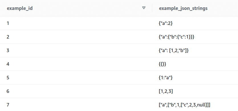
The following is the code to create a table and then load the data.
Create table test_json_functions(
example_id int,
example_json_strings varchar(max) --to load JSON data
);

copy test_json_functions --redshift code
from 's3://semistrcuturedbucket/test_json.csv'
iam_role 'arn:aws:iam::763031525305:role/myRedshiftRole'
CSV DELIMITER '|' QUOTE as '`' ;
JSON-SQL Functions supported by Redshift
- IS_VALID_JSON
This function is used to validate the inputted JSON string. Returns true if the string is valid, otherwise returns false.
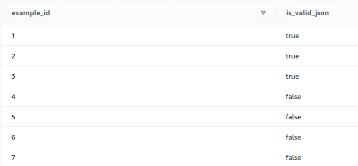
select example_id, is_valid_json(example_json_strings) from test_json_functions;
Output:
It can be seen from the input that the records 6 and 7 are JSON arrays and hence is_valid_json function returns false. To validate JSON arrays, the next function in the list is used.
2. IS_VALID_JSON_ARRAY
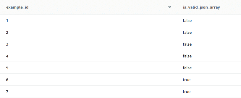
This function is used to validate the inputted JSON arrays. Returns true if the input array is valid, else returns false.
select example_id, is_valid_json_array(example_json_strings) from test_json_functions;
Output:
3. JSON_ARRAY_LENGTH
This function returns the number of elements in the outer array of a JSON string if the string is valid, otherwise it returns error. If the null_if_invalid argument is set to true and the JSON string is invalid, the function returns NULL instead of returning an error.
Syntax: json_array_length(‘json_array‘ [, null_if_invalid ] )
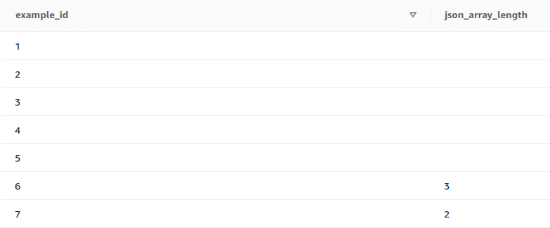
select example_id, json_array_length(example_json_strings, true) from test_json_functions;
Output:
It can be seen from the output that the first 5 elements are JSON arrays and we have specified null_if_invalid argument to ‘true’, hence this function returns null for the first 5 records.
4. JSON_EXTRACT_ARRAY_ELEMENT_TEXT
This function returns a JSON array element at specified index in the outermost array of a valid JSON string. The first element in an array is at position 0. If the index is negative or out of bound, JSON_EXTRACT_ARRAY_ELEMENT_TEXT returns an empty string. If the null_if_invalid argument is set to true and the JSON string is invalid, the function returns NULL instead of returning an error.
Syntax: json_extract_array_element_text(‘json string‘, pos [, null_if_invalid ] )
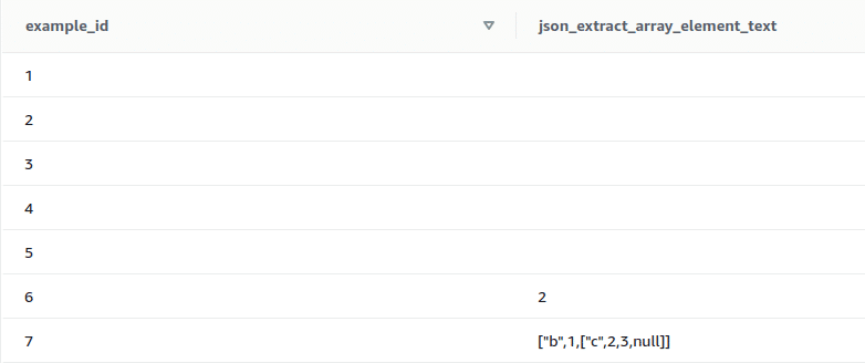
In the following example, the pos argument is set to 1 so this function returns the 2nd element in the array.
select example_id, json_extract_array_element_text(example_json_strings, 1, true) from test_json_functions;
Output:
5. JSON_EXTRACT_PATH_TEXT
This function returns the value for the key:value pair referenced by a series of path elements in a JSON string. The JSON path can be nested up to five levels deep. Path elements are case-sensitive. If a path element does not exist in the JSON string, JSON_EXTRACT_PATH_TEXT returns an empty string. If the null_if_invalid argument is set to true and the JSON string is invalid, the function returns NULL instead of returning an error.
Syntax: json_extract_path_text(‘json_string‘, ‘path_elem‘ [,’path_elem‘[, …] ] [, null_if_invalid ] )
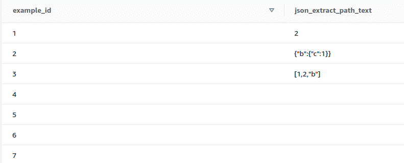
select example_id, json_extract_path_text(example_json_strings,'a’,true) from test_json_functions;
Output:
It can be seen from the output that the last four records are null as they are invalid JSON strings.
Limitations of JSON functions:
- JSON uses UTF-8 encoded text strings, so JSON strings can be stored as CHAR or VARCHAR data types in Amazon Redshift. Redshift’s VARCHAR data type supports a maximum size of 64KB.
- Redshift checks for valid JSON text every time when it executes any JSON function on JSON text field. This overhead of validating the input data increases the execution time of JSON functions.
- JSON is not a good choice for storing larger datasets because by storing disparate data in a single column, JSON does not use the Amazon Redshift column store architecture.
- JSON_EXTRACT_PATH_TEXT function can only return the JSON text which nested up to five levels.
- Redshift does not support any function to unnest or flatten the nested JSON arrays. In order to achieve this, we will have to use JSON_EXTRACT_PATH_TEXT function to load the array which we want to flatten in one column. Then we can use the JSON_ARRAY_LENGTH and JSON_EXTRACT_ARRAY_ELEMENT_TEXT functions to extract the data from JSON arrays. Thus, it becomes inconvenient to convert the JSON data into a relational table format.
For a practical comparison of how another modern platform handles deeply nested JSON including array expansion and flattening, see our detailed Databricks JSON guide Read Parse Query and Flatten Data.
FlowForward.
All Things Data Engineering
Straight to Your Inbox!
To summarize, Redshift has limited functions to query JSON data. Also, these functions cannot process the JSON data efficiently. Hence, the Redshift JSON data should be converted into the standard relational table format to use it efficiently.
Querying JSON data in Snowflake
Snowflake has extensions to SQL to reference the internal schema of the data. With these extended functions, we can query the JSON components and join it with the columns in other tables, as if it is in the standard relational format.
Let’s see how Snowflake simplifies the JSON data processing without converting the JSON data into relational format.
Input data:
{
    "fullName": "Johnny Appleseed",
    "age": 42,
    "gender": "Male",
    "phoneNumber": {
   	 "areaCode": "415",
   	 "subscriberNumber": "5551234"},
    "children": [{"name": "Jayden","gender": "Male","age": "10"},
{"name": "Emma","gender": "Female","age": "8"},
{"name": "Madelyn","gender": "Female","age": "6"}],
    "citiesLived": [{"cityName": "London","yearsLived": ["1989", "1993", "1998", "2002"]}, {"cityName": "San Francisco","yearsLived": ["1990", "1993", "1998", "2008"]}, {"cityName": "Portland","yearsLived": ["1993", "1998", "2003", "2005"]}, {"cityName": "Austin","yearsLived": ["1973", "1998", "2001", "2005"] }]
}
Let’s create a table and load some data into it. We will use parse_json() function which converts text into VARIANT data.
create or replace table json_demo (v variant);

insert into json_demo select parse_json( '{ "fullName": "Johnny Appleseed", "age": 42, "gender": "Male", "phoneNumber": { "areaCode": "415", "subscriberNumber": "5551234" }, "children": [ { "name": "Jayden", "gender": "Male", "age": "10" }, { "name": "Emma", "gender": "Female", "age": "8" }, { "name": "Madelyn", "gender": "Female", "age": "6" } ], "citiesLived": [ { "cityName": "London", "yearsLived": [ "1989", "1993", "1998", "2002" ] }, { "cityName": "San Francisco", "yearsLived": [ "1990", "1993", "1998", "2008" ] }, { "cityName": "Portland", "yearsLived": [ "1993", "1998", "2003", "2005" ] }, { "cityName": "Austin", "yearsLived": [ "1973", "1998", "2001", "2005" ] } ] }');

Select * from json_demo;
Output:

Now, let’s start querying the data. Suppose we want to fetch the full name from the JSON data that we have loaded.
select v:fullName from json_demo;
Where:
v = the column name in the json_demo table (from our create table command)
fullName = attribute in the JSON schema
v:fullName = notation to indicate which attribute in column “v” we want to select
This is similar to the dot notation(table.column) in SQL. Here, we use colon to reference the JSON field name from the variant column.
Output:

If we look at the above output, we can see the double quotes around the full name. We can cast it to the string format which will make it the same as the output we get after querying standard relational tables. We can also give an alias for the column name.
select v:fullName::string as full_name,
   v:age::int as age,
   v:gender::string as gender from json_demo;
:: is the notation used to cast the data.
Output:
The output looks the same as if it is from the structured data. This was all about querying first level data. Now, let’s see how we can query nested data. If we look at the input data, fullName, age, gender, phoneNumber are first level fields. phoneNumber has a nested structure and it contains an areaCode and a subscriberNumber The dot operator is used to reference this nested data. 
Select v:phoneNumber.areaCode::string as area_code, v:phoneNumber.subscriberNumber::string as subscriber_number from json_demo;
Output:

What happens to the queries if the structure changes on the fly?
If the extra field called extentionNumber is added in the phoneNumber, then what will happen to the above query?
{ "fullName": "Johnny Appleseed", "age": 42, "gender": "Male", "phoneNumber": { "areaCode": "415", "subscriberNumber": "5551234", "extensionNumber": "24" },...
The previous query will work the same as it was. Now, if we want to retrieve the extensionNumber then we need to add it in the query.
Select v:phoneNumber.areaCode::string as area_code,    v:phoneNumber.subscriberNumber::string as subscriber_number,
v:phoneNumber.extensionNumber::string as extension_number from json_demo;
If the reverse happens and some attribute is dropped, then the query will simply return NULL value. Thus, the snowflake is flexible and can easily accommodate the dynamic changes.
How to handle arrays of data?
Now, let’s see how we can deal with the arrays of data within the document. In this case, we have a Children array.
select array_size(v:children) as number_of_children from json_demo;
There is a function called array_size() which returns the number of elements in the array.
Output:

If we want to retrieve the individual elements, then the following query can be used. For this, we will use the dot notation along with the reference for row number in the square brackets.
select v:children[0].name from json_demo union all
select v:children[1].name from json_demo union all
select v:children[2].name from json_demo;
Output:

Snowflake has a special function called flatten(), which can be used to convert semi-structured data to a relational representation. FLATTEN allows us to determine the structure and content of the array on the fly.
Select	f.value:name::string as child_name,
f.value:gender::string as child_gender,
f.value:age::string as child_age
from json_demo,table(flatten(v:children)) f;
Output:

This is how we can get all the array sub-columns using flatten() in the format same as a relational table.
This can be combined with the first level element such as the full name of the parent.
Select	v:fullName::string as parent_name,
f.value:name::string as child_name,
f.value:gender::string  as child_gender,
f.value:age::string as child_age
from json_demo,table(flatten(v:children)) f;
Output:

How to handle multiple arrays at once
Snowflake allows us to pull the data from multiple arrays at once. The following is the example for the same. We are retrieving the data from citiesLived and children arrays from the input.
Select	v:fullName::string as Parent_Name,
array_size(v:citiesLived) as Cities_lived_in,
array_size(v:children) as Number_of_Children
from json_demo;
Output:

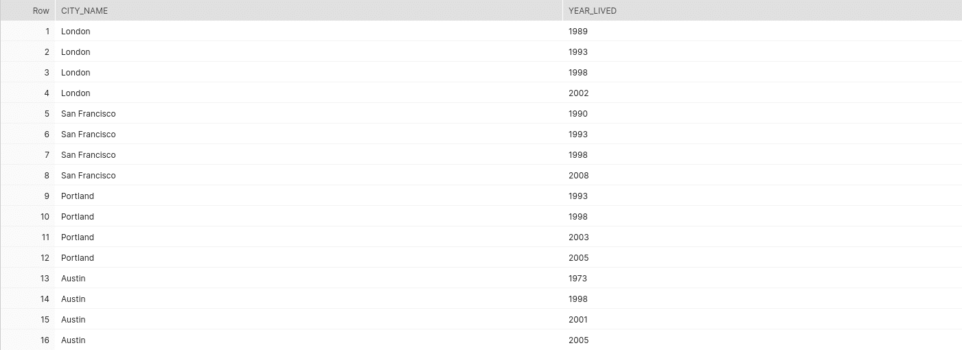
We can also retrieve data from the array which is nested inside another array. For example, the citiesLived array contains yearsLived array. The following query shows how we can retrieve data from the yearsLived array.
Select	cl.value:cityName::string as city_name,
yl.value::string as year_lived
from json_demo,
table(flatten(v:citiesLived)) cl,table(flatten(cl.value:yearsLived)) yl;
To retrieve that data, we need to add a second FLATTEN clause that transforms the yearsLived array within the FLATTENed citiesLived array.
Output:
How can we perform standard SQL aggregation and filter data?
Using Snowflake, we can even execute standard SQL aggregations on the semi-structured data. The following query will show how to perform aggregations on the JSON data.
Select cl.value:cityName::string as city_name,
count(*) as year_lived
from json_demo,table(flatten(v:citiesLived)) cl,table(flatten(cl.value:yearsLived)) yl group by 1;
Output:

Apart from the standard aggregate functions, we can use window functions such as LEAD, LAG, RANK, and STDDEV.
Snowflake also supports the use of WHERE clause to filter the JSON data. The following example demonstrates how we can use WHERE clause to filter required rows.
select  cl.value:cityName::string as city_name,
    	count(*) as years_lived
from json_demo,table(flatten(v:citiesLived)) cl,table(flatten(cl.value:yearsLived)) yl
where city_name = 'Portland'
group by 1;
Output:

To make it easier to read the SQL, we can even reference the alias city_name in the predicate. You can also use the full specification cl.value:cityName
To summarize, Snowflake offers a set of functions such as parse_json(), flatten(), array_size(), which help in dealing with the multilevel nested JSON data without converting it to the relational format. Also, we can cast the retrieved data using the :: operator. The colon(:) notation can be used to retrieve first level elements. We can even use aggregate functions and WHERE clause to filter the data.
Automatically convert any JSON to a relational format in Snowflake and Redshift
Both Snowflake and Redshift have limitations when converting JSON data to a readable database format.
- Individual JSON documents must not exceed a certain size.
- Engineers still need to write code to manually convert the JSON. This is not a problem for simple JSON documents. However, once you have a certain complexity, deep nesting, and a large number of different JSON documents, this overhead becomes significant.
For those limitations and scenarios, we have come up with Flexter. Flexter automatically converts any JSON to a readable format in seconds. The conversion process is fully automated. No need for niche skills and long development life cycles.
Flexter not only automates the conversion process, it also simplifies the output for downstream consumption. Flexter uses two optimization algorithms, and you can read about the details in the following blog post (in the context of XML)
For scenarios where you need JSON data loaded into a relational database (JSON → SQL), Flexter can infer the schema, generate the corresponding DDL, and automatically load the data into targets such as Redshift or Snowflake, significantly accelerating deployment. You can learn more about how Flexter handles JSON-to-SQL conversion in our detailed JSON to SQL guide
Rapid, seamless access to complex JSON data for advanced, evidence-based analytics
- More time – cut hours of manual work to minutes with rapid, automated data conversion
- Less manpower – remove the need to hire expensive data specialists to help unlock data
- Lower costs –retain more of your budget to deliver real value to the business
- Reduced risk – lower the threat of exceeding budgets and missing project SLAs
- Quicker decisions – obtain critical data for essential decision-making more rapidly
- Readable output
Conclusion
In this document, we have compared Amazon Redshift and Snowflake platforms based on their ability to load and query JSON data.
To load the data in Amazon redshift, we need to analyze the schema of the source data and manually create the target table based on the analysis. COPY FROM JSON options, parse the input JSON string based on the jsonpath file or the column names in the target table. The JSON strings need to be stored into CHAR or VARCHAR data types and the VARCHAR data type supports a maximum size of 64KB. They have also introduced a new data type called SUPER to load the data directly into a single column without worrying about its schema. But this data type can be used only for testing and not in the production environments. The SUPER data type only supports up to 1MB of data for individual rows.
Snowflake has a new data type called VARIANT that allows JSON data to be loaded, as it is, into a column in a relational table. Thus, you don’t need to worry about the schema of the source data. Even if the schema changes on the fly, we don’t need to change the code to load the changed schema. Also, VARIANT provides the same performance as all the standard relational data types. The only limitation is that the VARIANT data type imposes a 16 MB (compressed) size limit on individual rows.
Amazon Redshift supports limited functions to deal with JSON data. These functions can be used to find the number of elements in the JSON arrays, specific elements in the array based on position, the element in the JSON string based on the specified path. Redshift does not support a function to flatten the nested JSON arrays.
On the other hand, Snowflake provides a lot of functionalities to directly query the JSON data without converting it to the relational format. It provides a FLATTEN function to expand the nested JSON objects into individual JSON objects which makes it easy to deal with nested objects. We can even use aggregate functions and WHERE clause to filter the data. We can say that Snowflake is a very powerful and efficient platform to deal with JSON data.


