JSON to SQL & Database – Load, Query, Convert (Guide)

If you work with databases today, you’ve almost certainly come across the JSON data format.
It powers everything from API integrations to event streams and user data, and it’s no longer just for NoSQL systems.
Modern relational databases can now store and query JSON directly, merging flexibility with structure.
This means you no longer need to overthink which schema to apply, or how to squeeze JSON into traditional SQL tables.
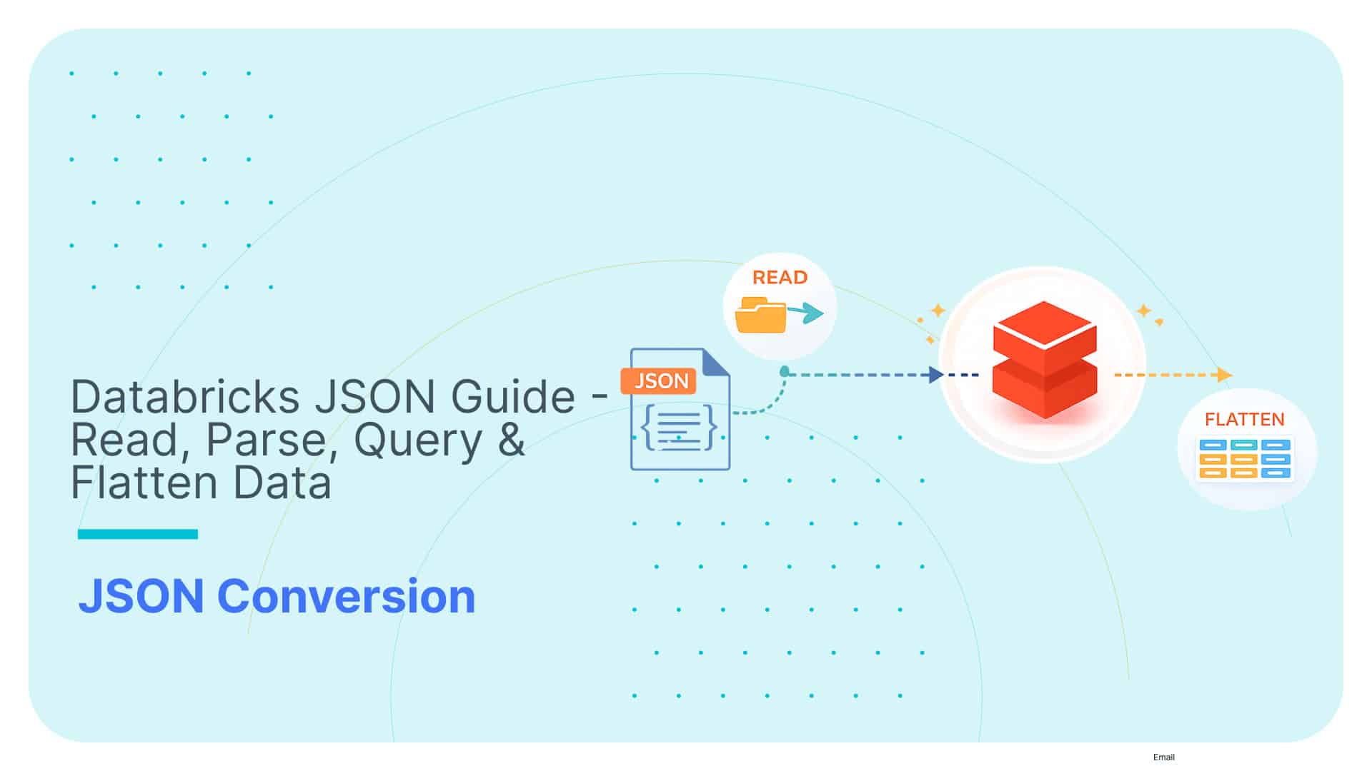
If you’re also working with JSON on modern data platforms like Databricks, check out our Databricks JSON Guide Read Parse Query and Flatten Data for step-by-step coverage on reading, parsing, querying, and flattening JSON.
With today’s engines, you can choose to apply structure when you write (schema on write), when you read (schema on read), or adopt a hybrid approach that combines the best of both worlds.
In this article, I’ll break down how to work with JSON in SQL databases: how to load it, store it, query it, and even convert it into relational tables.
We’ll look at manual and SQL-native approaches, discuss their limitations, and explore how automation tools like Flexter simplify the entire process.
TL;DR for those in a hurry:
- I’ll show you how to load JSON into modern databases as-is: via external tables, batch loaders, streaming, or app inserts, and what to watch out for.
- You’ll see when to use schema on read versus schema on write, and how to combine both in hybrid architectures.
- I’ll walk you through querying and extracting JSON with SQL/JSON path functions across major engines.
- You’ll discover your options to convert JSON to relational models, and how Flexter can automate schema creation and JSON to SQL conversion.
Let’s kick this off with some options for loading your source JSON to a database.
Use Flexter to turn XML and JSON into Valuable Insights
- 100% Automation
- 0% Coding
How to insert JSON into SQL tables
One of the first things to know about working with JSON in a database is that you don’t need to convert it into SQL tables right away.
Most modern databases support native JSON storage, so that you can load and query JSON with minimal setup.
This works perfectly for semi-structured data, API payloads, event logs, or documents that don’t fit neatly into rows and columns.
Next, I’ll provide you with the fundamentals of loading JSON data into a database.
TL;DR
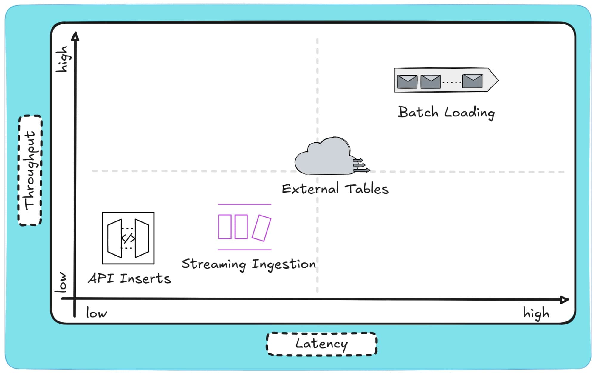
This section covers the four main ways to load JSON into a database: External Tables (for exploration), Streaming Ingestion (for real-time), Batch Loading (for high volume), and API Inserts (for transactional data) . Each method offers a different trade-off between speed (latency) and volume (throughput).
Once your data is loaded, you must decide how to store it; if you’re ready to skip ahead, see the next section on storage approaches, or check the Glossary for key terms.
The ingestion challenge for JSON to SQL
The central question for data architects isn’t just if a system can handle JSON, but how it does so across a spectrum of competing requirements.
This is commonly referred to as the ingestion challenge and is a central concept when loading JSON into a database.
Every ingestion strategy involves trade-offs across two critical dimensions:
- Latency: the delay between data generation and when it becomes available for querying. This can range from milliseconds in real-time systems to hours or even days in batch processes.
- Throughput: the amount of data processed per unit of time, which becomes crucial for large-scale migrations or high-volume event streams.
These two forces are often in tension; improving one can hurt the other.
For example, maximising throughput through bulk batch loads inevitably increases latency, while low-latency streaming can strain scalability.
To navigate these trade-offs, different systems adopt distinct ingestion strategies, each tuned for a specific balance of speed, scale, and operational complexity.
Over time, four primary paradigms have emerged for loading JSON into databases:
- External Tables: Query JSON files directly from (object) storage without loading them into the database.
- Batch Loading: Ingest large JSON datasets periodically using commands like COPY, Oracle’s SQL Loader, SQL Server’s BCP, COPY INTO, or bq load.
- Streaming Ingestion: Push JSON data continuously from message queues for near-real-time use cases.
- API or Application Inserts: Write JSON directly from applications or microservices for transactional workloads.
And here’s a visual of how these four methods correlate to Latency and Throughput:
In the next section, I’ll break down each of these ingestion methods in more detail, explaining when to use them, their limitations, and how different databases implement them in practice.
Pro tip
Loading JSON to a database is very different from converting JSON to a database.
When you load JSON, you are simply storing it as-is, in its raw, semi-structured form, and often untouched.
When you convert JSON, you are transforming it into a relational model with defined tables, keys, and data types.
Both have their place, but only conversion gives you a query-optimised database ready for analytics and integration.
Method 1: Exploratory Querying with External Tables
When you are starting out with new JSON data, the easiest option is often not to load it at all.
External tables let you query JSON directly where it resides, whether that is in S3, Azure Blob Storage, Google Cloud Storage, or any other object store, without physically ingesting it into the database.
It is quick to set up and great for discovery, though not designed for high-performance or transactional use.
Here’s how this process looks in a diagram:
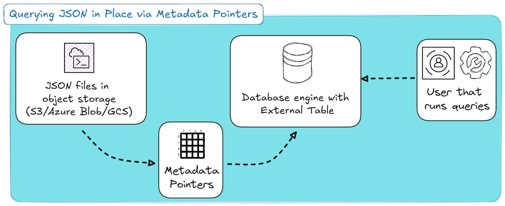
How It Is Implemented Across Ecosystems
Most modern databases and analytics engines now support external tables with metadata pointers, which are lightweight references that link table definitions to underlying JSON files without copying or parsing them upfront.
- Snowflake: CREATE EXTERNAL TABLE uses metadata pointers to JSON files in S3 or Azure, storing only column mappings and file locations.
- Amazon Redshift Spectrum: Queries JSON in S3 through AWS Glue, which acts as the metadata catalog.
- Google BigQuery: Defines external tables on JSON files in Cloud Storage, using metadata references for dynamic schema inference.
- Azure Synapse: Uses OPENROWSET or PolyBase to read JSON from Blob Storage through external metadata sources.
- Databricks: Uses Delta Live Tables to define external views that point to JSON data in the data lake.
- PostgreSQL / Trino / Presto: Use foreign data wrappers (FDWs) or connectors to create virtual tables backed by metadata pointers to files.
Across all platforms, the principle is the same: query JSON through lightweight metadata instead of full ingestion.
Pros and Cons
|
Pros |
Cons |
|---|---|
|
No ingestion required, query JSON directly from storage. |
Slower performance on large or deeply nested datasets. |
|
Cost-efficient, compute only when queried. |
Limited indexing and optimisation. |
|
Ideal for schema discovery and data profiling. |
Schema inference can vary between queries. |
|
Uses lightweight metadata pointers for efficient access. |
Not suitable for frequent queries or production workloads. |
Use cases:
- Schema Discovery and Data Exploration
Analysts can use external tables to inspect and understand new JSON structures, such as event streams or API dumps, before deciding how to model or normalise them in SQL.
- Cost-Efficient Validation and Prototyping
Engineers can quickly validate or profile large JSON datasets directly in cloud storage, eliminating the need to build ingestion pipelines, making this approach ideal for exploratory analysis or sandbox environments.
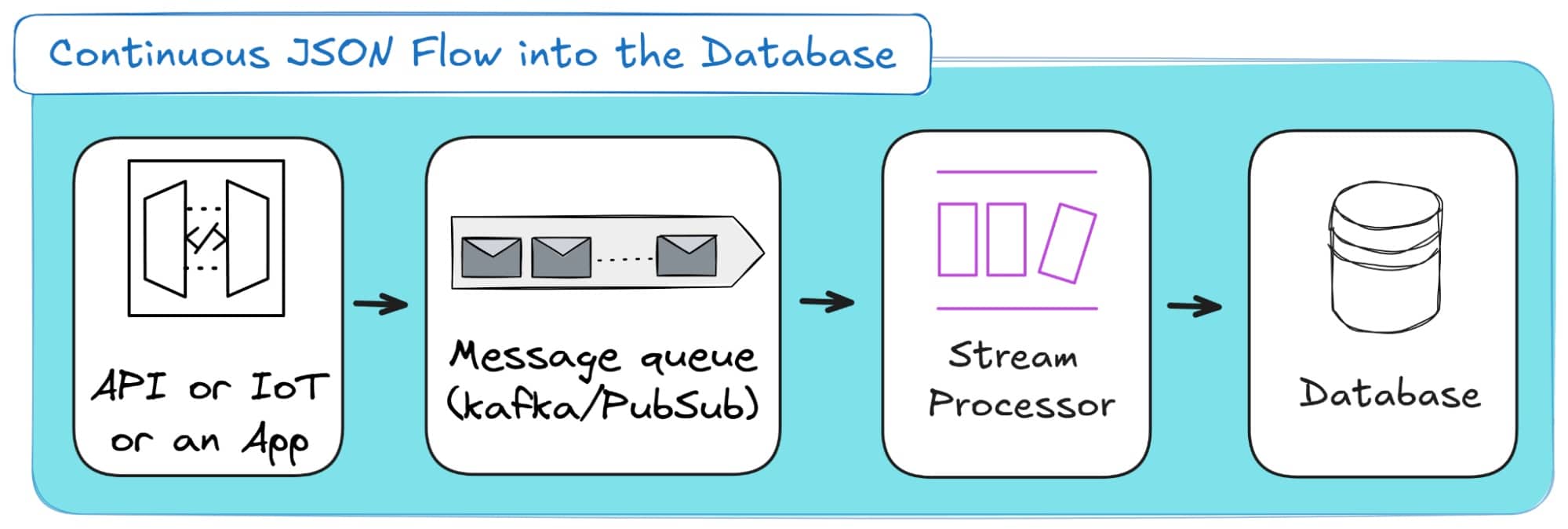
Method 2: Real-Time Ingestion via Streaming Architectures
If external tables are about querying JSON where it lives, real-time ingestion is about moving it the moment it is created.
Instead of reading static JSON files from storage, streaming architectures continuously capture and deliver JSON data as events occur.
This approach is designed for low-latency ingestion, where every second counts.
Data flows from sources such as APIs, IoT sensors, or applications through message queues and stream processors into your target database or data warehouse.
It is the natural next step when your workload evolves from exploratory querying to operational, always-on data pipelines.
The process works as follows:
How It is Implemented Across Ecosystems
Every major cloud and analytics platform supports streaming ingestion for JSON.
While the technologies differ, the idea remains the same: capture, transport, and write JSON records in near real-time.
Here are some options:
- Snowflake: Uses Snowpipe Streaming to ingest JSON from message queues or cloud storage directly into tables.
- BigQuery: Offers Streaming Inserts API and integration with Pub/Sub for continuous ingestion of JSON payloads.
- Amazon Redshift: Connects with Kinesis Data Streams or Firehose for real-time delivery of JSON data.
- Azure Synapse: Ingests JSON via Event Hubs or Stream Analytics, pushing data into staging or target tables.
- Databricks: Uses Autoloader to process and store incoming JSON streams as Delta tables.
- PostgreSQL and MySQL: Often integrated with tools such as Kafka, Debezium, or Change Data Capture (CDC) to propagate JSON updates from operational systems.
Pros and Cons
|
Pros |
Cons |
|---|---|
|
Near real-time data availability. |
Requires more complex infrastructure and monitoring. |
|
Enables continuous, event-driven pipelines. |
Schema evolution can be difficult to manage. |
|
Reduces latency compared to batch or scheduled loads. |
Higher operational and scaling costs. |
|
Perfect for transactional and high-velocity JSON data. |
Complexity grows with system volume. |
Use Cases:
- Operational Monitoring and Alerting
Ideal for systems tracking transactions, telemetry, or user activity. JSON events are streamed into analytics tables or dashboards as they happen, enabling real-time alerts and performance insights.
- Change Data Capture (CDC) and System Synchronisation
Many modern systems use JSON to transmit incremental updates between microservices or databases. Streaming ingestion ensures these updates are captured and reflected across environments within seconds, maintaining consistency.
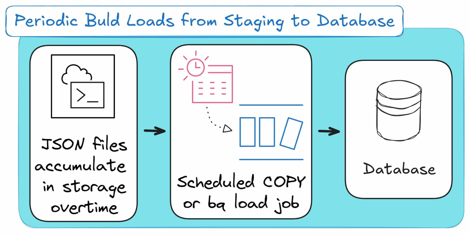
Method 3: High-Throughput Bulk Loading with Batch Ingestion
If streaming ingestion is about constant motion, batch loading is about efficiency through bulk loading rather than one-by-one processing.
Instead of pushing every JSON record as it arrives, data is collected over time and then ingested into the database in larger, periodic batches.
This approach optimises for throughput rather than latency. It reduces the overhead of constant writes and is ideal for systems where slight delays are acceptable (for example, in data warehousing and BI).
Batch loading remains one of the most common methods for importing large volumes of JSON data into databases and data warehouses, as it strikes a balance between performance, cost, and simplicity.
Here’s how this method looks on a conceptual level:
How It Is Implemented Across Ecosystems
Batch loading is universally supported across data platforms, often through dedicated bulk utilities or managed services.
- Snowflake: Uses COPY INTO to load staged JSON files from S3, Azure, or GCS into tables, with automatic parsing and semi-structured type support.
- Amazon Redshift: The COPY command loads JSON data from S3 or DynamoDB using JSONPaths for field mapping and transformation.
- BigQuery: Ingests JSON files directly from Cloud Storage through the bq load command, supporting both newline-delimited and array-based JSON.
- Azure Synapse: Leverages PolyBase or COPY INTO for high-performance parallel loading from Blob Storage.
- Databricks: Uses Autoloader jobs to read JSON from data lakes and write to Delta tables.
- PostgreSQL and MySQL: Support bulk ingestion through COPY FROM, LOAD DATA INFILE, or client libraries for JSON text.
Across all ecosystems, the pattern is the same: stage JSON files in a reliable storage layer, then load them into a target system using parallelised bulk commands.
Pros and Cons
|
Pros |
Cons |
|---|---|
|
High throughput and scalability. |
Higher latency between data generation and availability. |
|
Efficient for large JSON volumes. |
Schema mismatches can impact the entire batch. |
|
Simple, reliable and easy to schedule. |
Requires staging infrastructure and batch orchestration. |
|
Cost-efficient and robust compared to real-time ingestion. |
Limited flexibility for time-sensitive data. |
Use Cases:
- Data Warehousing and ETL Pipelines
Batch loading is the backbone of most ETL workflows. Large JSON exports from APIs or logs can be processed daily or hourly, transformed, and written into relational tables for analytics.
- Historical Backfills and Archive Loads
When onboarding new datasets or migrating systems, batch loading allows teams to process months or years of historical JSON data efficiently without impacting live systems.
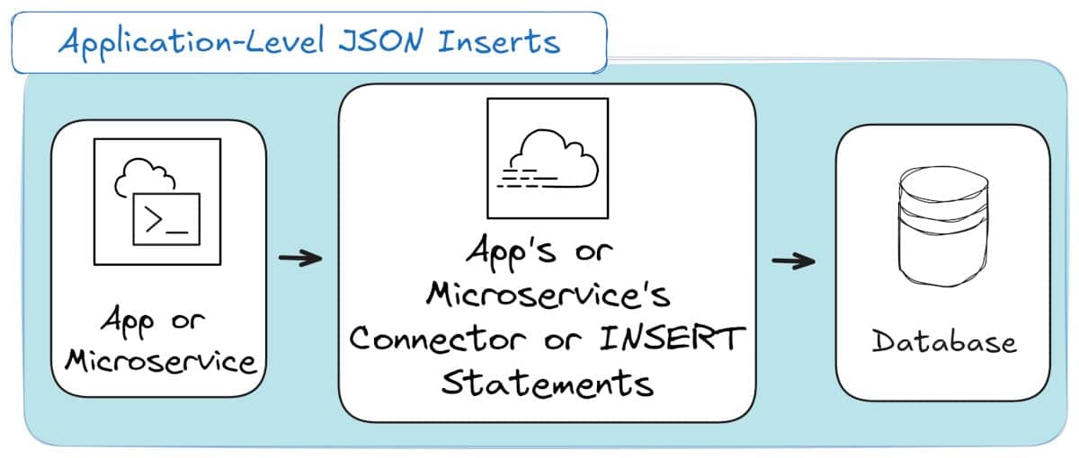
Method 4: Transactional Integrity with API-Driven Inserts
While batch loading focuses on throughput, API or application-based inserts focus on immediacy and control.
Instead of loading JSON from files or streams, the application itself writes JSON directly into the database, one record or small batch at a time.
This method is common in transactional systems, microservices, and application backends where new JSON data is created continuously and must be available instantly.
It trades efficiency for precision; perfect for scenarios where every insert matters and must be confirmed in real time.
And here’s a high-level overview, if you’re the visual type of person:
How It Is Implemented Across Ecosystems
Most databases and data platforms provide APIs, SDKs, or connectors that make inserting JSON directly from applications straightforward.
- PostgreSQL and MySQL: Support direct INSERT operations into JSON or JSONB columns using SQL commands or client libraries such as psycopg2, SQLAlchemy, or JDBC.
- SQL Server: Allows INSERT statements with raw JSON values or uses OPENJSON for more structured inserts.
- Snowflake: Supports inserts through Snowflake Connector APIs and can automatically cast JSON strings into its VARIANT type.
- BigQuery: Accepts direct inserts using the BigQuery Streaming API for transactional data.
- Databricks: Applications can write JSON via JDBC, Spark Structured Streaming, or Delta tables APIs for immediate persistence.
- NoSQL systems such as MongoDB or Couchbase mostly rely on this approach, using native document APIs for JSON storage. MongoDB has introduced bulk ingestion and streaming as well.
Pros and Cons
|
Pros |
Cons |
|---|---|
|
Low latency and immediate data availability. |
Limited throughput, not ideal for bulk ingestion. |
|
Full control from the application layer. |
Higher load on transactional databases. |
|
Ensures consistency for each insert. |
Requires more connection management and retries. |
|
Ideal for event-driven or operational systems. |
Can increase storage fragmentation over time. |
Use Cases:
- Microservices and Event APIs
JSON is the standard payload format in modern APIs. Application-based inserts allow microservices to persist events, logs, or configuration updates directly into the database in real time, without waiting for ETL or staging.
- Operational Systems with Immediate Consistency
Financial systems, booking platforms, and inventory applications often need every JSON transaction written immediately. Application-level inserts ensure that data is stored and queryable the moment it is created.
Comparison table
To facilitate decision-making, the following table provides a comparative summary of the four ingestion methods across key architectural dimensions.
|
Dimension |
External Tables |
Streaming Ingestion |
Batch Loaders (COPY) |
API-Driven Inserts |
|---|---|---|---|---|
|
Primary Use Case |
Ad-hoc exploration, data lake querying, ETL source |
Real-time analytics, CDC, event-driven apps |
Bulk data migration, periodic ETL |
Operational applications, systems of record |
|
Latency Profile |
High (seconds to minutes) |
Very Low (milliseconds to seconds) |
Very High (minutes to hours) |
Low (milliseconds to seconds) |
|
Throughput Profile |
Low-to-Medium (per query) |
Low (sustained stream) |
Very High (burst) |
Low (per transaction) |
|
Operational Complexity |
Low |
High |
Medium |
Low |
|
Relative Cost |
Low (pay-per-query on cheap storage) |
High (requires managed broker/processing) |
Low – Medium (compute for load jobs) |
Low (part of application infrastructure) |
Approaches to Storing JSON in a Database
In this section, I’ll discuss your two options if you want to store JSON in a database, without first converting it to a table or a relational model.
In this case, there are essentially two schools of thought: treat your JSON as plain text or treat it as if it was structured data.
The first is fast to implement but slow to query; the second takes a bit more setup but performs far better in the long run.
TL;DR
This section outlines your two main storage choices: Textual Storage (TEXT or VARCHAR) preserves the exact JSON string but is slow to query. Binary Storage (jsonb, VARIANT) parses the JSON on ingestion, enabling fast, indexed querying .
After storing your data, the next step is querying it; you can skip to the next section to learn about querying JSON in SQL, or visit the Glossary to understand these concepts.
Option 1: Textual (String-Based) Storage
This is the simplest approach. You store JSON as-is, usually in a TEXT, CLOB (Oracle), VARCHAR(MAX), or even JSON column. The database saves an exact copy of the input string, including whitespace.
The upside? Perfect fidelity. The JSON is stored exactly as received, which can be important for audit or archival use cases.
The downside, you ask? Bad query performance. Every time you query a key or nested field, the database has to parse the entire string again. Indexing is almost impossible unless you manually extract fields into columns.
You can think of this as the “junk drawer” model; everything fits, but good luck finding it later.
Option 2: Binary (Decomposed) Storage
Modern databases like PostgreSQL (jsonb), Oracle (JSON data type), MySQL (JSON), Snowflake (VARIANT), and Redshift (SUPER) take a smarter route.
They parse the JSON once on ingestion and store it in a binary, tree-like structure.
This gives the database a semantic understanding of the JSON hierarchy, meaning it can navigate directly to a key, index specific paths, and skip costly reparsing.
You lose some cosmetic fidelity (such as whitespace and key order), but you gain significant performance and indexing advantages.
Pro tip
If you’re working with XML instead of JSON, the same trade-off applies: structure versus fidelity.
Check out XML to Database Converter – Tools, Tips, & XML to SQL Guide to see how Flexter automates schema inference and conversion for XML.
Choosing the Right Model
For small datasets or archival storage, textual JSON is fine.
But for querying, joining, or analysing semi-structured data, the decomposed binary model wins every time.
It’s also the foundation for advanced features like path-based indexing, schema inference, and automatic JSON to SQL schema generation.
And here’s a comparison table to sum up the JSON storage options:
|
Feature |
Textual Storage (json) |
Binary Storage (jsonb, VARIANT, SUPER) |
|---|---|---|
|
Storage Type |
Raw text/string. |
Parsed binary tree. |
|
Write Speed |
Fast. |
Slightly slower (due to parsing). |
|
Read Performance |
Slow (requires reparsing). |
Fast (pre-parsed, direct access). |
|
Indexing |
Limited/manual extraction. |
Native path and value indexing. |
|
Data Fidelity |
Preserves formatting, key order, duplicates. |
Discards formatting, reorders keys. |
|
Use Case |
Archival, logging, audit. |
Querying, analytics, ETL, data warehouse. |
Pro tip
Querying JSON in SQL (JSON path, UNNEST/FLATTEN)
Once your JSON data is loaded and stored in the database, the next challenge is understanding how to query and extract it effectively.
Modern SQL engines have evolved to handle JSON natively, giving you the flexibility to treat it in multiple ways.
This means that you don’t necessarily have to convert all of your data to SQL tables when writing to the database (schema on write), or when retrieving the data (schema on read).
You can mix these two approaches and follow a “hybrid approach”.
TL;DR
This section details how to use SQL/JSON path functions to access, extract, and filter data directly within your JSON columns. It also covers performance indexing and using FLATTEN or UNNEST to turn nested arrays into queryable rows.
While querying is flexible, you often need to permanently convert your JSON; learn how in the next section on converting JSON to tables, or look up any unfamiliar terms in the Glossary.
Under the hybrid approach, you may decide to not only to load your JSON into the database, but also to convert it (all of it or parts of it). You may convert your JSON to a relational schema (by normalising) or to a One Big Table (OBT) by flattening it.
Together, these approaches form what I call “the unifying model” for working with JSON in SQL.
This “flexible continuum” allows you to store, access, and transform data according to your needs rather than your database’s limitations.
At its core, working with JSON in SQL revolves around four key operations:
- Access: Locate and reference JSON objects or arrays,
- Extract: Retrieve specific values or attributes,
- Filter: Apply logical conditions to select subsets of data,
- Project: Shape and return the data in tabular or hierarchical form.
Together, these actions map to standard SQL commands extended with JSON operators, functions, and path expressions.
The SQL/JSON Path Language (ISO/IEC 9075)
To bring consistency across platforms, the SQL/JSON Path Language (ISO/IEC 9075) defines a standard syntax for navigating and extracting data from JSON documents.
It provides a common framework for how databases interpret JSON structures and values.
At the heart of this language are path expressions that define how to traverse and retrieve elements.
The syntax uses familiar JSON conventions, dots for property access, square brackets for arrays, wrapped within SQL expressions like JSON_VALUE, JSON_QUERY, or JSON_EXISTS.
The standard defines two path modes:
- Lax mode: Ignores missing fields and automatically typecasts values when possible.
- Strict mode: Fails if the expected path or value type is not found.
While the standard provides structure, each database vendor has implemented its own variant.
For instance, SQL Server uses JSON_VALUE and OPENJSON functions following Microsoft’s path conventions, while Oracle integrates the ISO/IEC 9075 model into its JSON_TABLE function and native IS JSON predicates.
Pro tip
Just as you can use SQL/JSON extensions to query, filter, and project JSON data into relational tables, SQL/XML applies the same principles to XML.
If you want to see how this works in practice with XML, check out my other post on How to Insert XML into SQL Tables with SQL/XML.
Both standards share the same idea: extending SQL so you can work seamlessly with semi-structured data alongside traditional relational models.
Advanced Filtering and Predicate Logic
Beyond simple extraction, the SQL/JSON Path Language also supports advanced filtering using logical and comparison operators.
You can use path filters that begin with a dollar sign ($) to define evaluation contexts, for example, filtering array elements by value, testing conditions, or checking for the presence of nested keys.
Predicates can evaluate numeric, textual, or structural conditions within JSON documents.
Combined with SQL clauses like WHERE, HAVING, or JOIN, they make it possible to filter JSON data just as you would relational tables.
This approach allows developers and analysts to perform fine-grained queries across both structured and semi-structured data within a single SQL statement.
Performance Optimisation through Indexing
Querying JSON at scale introduces performance considerations. JSON data is flexible but not naturally optimised for relational access patterns.
To compensate, most databases support specialised indexing mechanisms for JSON columns.
- PostgreSQL uses GIN indexes on jsonb columns to accelerate key lookups and containment queries.
- SQL Server can create functional indexes on expressions like JSON_VALUE to speed up repeated path queries, while Oracle provides dedicated JSON indexes designed for efficient path-based access.
- Snowflake uses micro-partitioning for efficient JSON scanning.
The general rule is simple: indexing JSON works best when you know which paths are queried frequently. This turns schema on read flexibility into near-schema-on-write performance.
Projecting JSON into Relational Structures
Another option with SQL/JSON comes when you need to project hierarchical or array-based JSON data into relational form.
Using ISO/IEC 9075 functions and vendor extensions, you can expand arrays into multiple rows and map their elements to table columns.
A common example is Snowflake’s LATERAL FLATTEN() command, which unpacks JSON arrays so that each item can be treated as an individual row.
Similarly, BigQuery’s UNNEST(), SQL Server’s OPENJSON, and Oracle’s JSON_TABLE achieve the same goal, turning nested or multi-level JSON into relationally accessible data.
While this topic overlaps with full conversion, here it serves as an analytical step: projecting JSON for temporary querying or lightweight denormalisation.
I will explore deeper conversion workflows in the next section.
Limitations and Pitfalls of SQL/JSON
Despite its maturity, SQL/JSON querying has a few caveats to keep in mind:
- Still, using SQL/JSON to handle JSON in your database is a lot of manual work: This means that you will still need the right skills, personnel and manhours to manually put together the manual SQL code that will handle your JSON and resulting SQL tables.
- Inconsistent syntax across vendors: While ISO/IEC 9075 defines a standard, real-world implementations vary in functions, operators, and path expressions.
- Schema drift challenges: When JSON structure changes, existing queries or indexes can break silently or return partial results.
- Performance overhead: Deeply nested or large JSON documents can cause expensive parsing operations if not properly indexed or flattened.
- Limited tooling support: Debugging JSON queries is still harder than debugging relational SQL, especially when working across multiple database systems.
In short, querying JSON in SQL has some strengths, but requires discipline. Treat JSON as a first-class citizen, but remember that it carries its own operational costs.
Pro tip
If you want to see how automated converters handle JSON conversion to relational schema for you, check out the Flexter JSON to SQL Database Converter.
It automatically interprets nested JSON paths, generates schema mappings, and even produces relational SQL output, all without writing a single path expression. Online, for free.
If you’ve already tested the Online Free Version of Flexter then read about the advanced features of Flexter Enterprise or even ask us for free trial!
Converting JSON to Database Tables
Next, I’ll present my three approaches for converting JSON to SQL, along with a comparison table to help you make an informed choice.
TL;DR
This section explains how to permanently transform JSON into a relational model. It details the manual approaches (using Python or native SQL) where you must design the schema and write the mapping code yourself. It then contrasts this with an automated tool like Flexter, which automates schema generation and conversion.
Knowing the how of conversion is key, but the strategy is just as important; skip ahead to learn about best practices and patterns, or consult the Glossary for definitions.
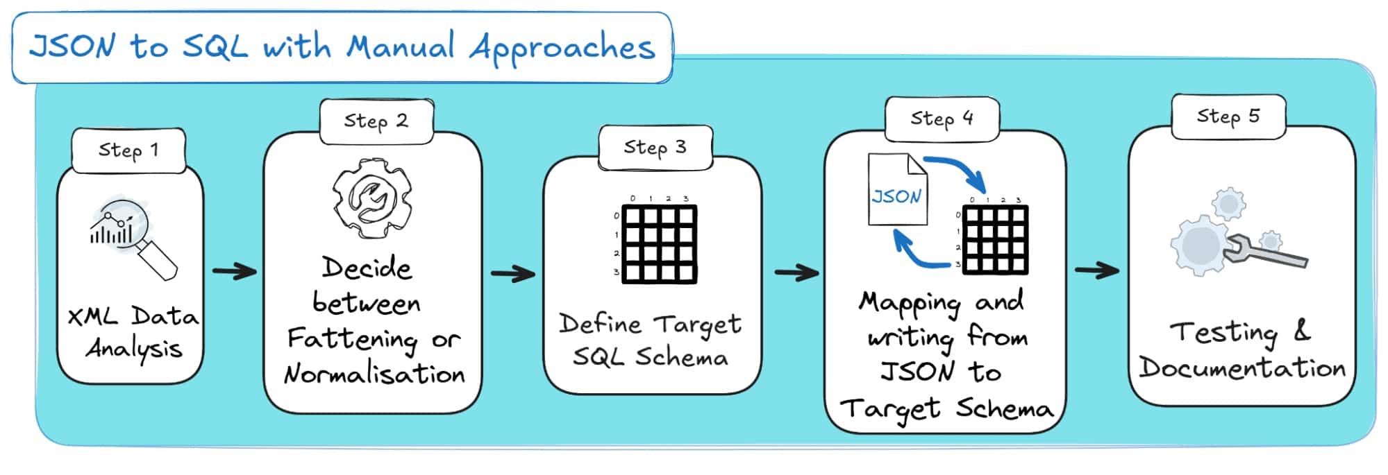
Manually converting JSON to Tables
The first two approaches that I would like to show you, fall under the umbrella of manual approaches for converting JSON to SQL.
Why are they called that? Because, unlike automated tools, you’re writing all of the conversion logic yourself in code.
If you decide to go hands-on with these approaches, you’ll quickly notice that it gives you control over every detail, but at the cost of more effort on your side.
Both approaches follow the same playbook; a series of key steps you’ll need to go through to get your JSON data into SQL.
Step 1: Analyse and understand your source JSON data.
Whenever I take the manual approach, my first step is to understand the JSON structure.
You should always check if the file is flat or nested, and spot parent-child relationships.
This makes a big difference when you’re working on something like a nested JSON to SQL table.
Without that analysis, your schema design process can quickly fall apart.
Step 2: Decide between Flattening vs. Normalisation
Here’s where beginners often take shortcuts.
If you’ve followed my section on Flattening and Denormalisation vs Normalisation, you’ve probably found out that it’s tempting to flatten everything into one wide table just to get things running.
While flattening may work in very simple cases of JSON to SQL table conversions, in most real-world JSON to DB table conversions, it won’t.
Once the dataset grows, flattening will create bloated tables full of NULL and redundant values.
In my experience, a normalised design, splitting into related tables, is far better for long-term maintainability.
Step 3: Decide on your target SQL schema modeling
Once you’ve completed preparatory steps 1 and 2, you need to design the target SQL schema.
This involves deciding on how many tables you’ll need, what their relationships will look like, and which fields belong where.
And if you’re normalising your source JSON (which is the correct approach), then you’ll also need to carefully define primary keys, foreign keys, and data types.
This is where the manual coding approach becomes tricky: you’re not just mapping fields one-to-one; you’re designing a relational structure that has to stand the test of time.
If you oversimplify, you’ll end up with bloated tables full of NULLs. If you over-normalise, you may struggle with complex joins and slow queries later.
Step 4: Manual mapping and writing
This is also a truly hands-on part.
This is where you need to align the raw JSON elements with the SQL tables and columns you designed in Step 3.
The upside? Coding the mapping yourself gives you the maximum flexibility; you decide exactly how fields get translated.
The downside, you ask? This step takes a considerable amount of manual effort.
In fact, I’ve seen projects stall for months while trying to get the mappings from the source JSON to the target tables right.
So be prepared for a lot of trial and error, debugging, and constant schema adjustments.
This is because you’ll often find that your first mapping isn’t perfect; you’ll need to refine it, rerun your scripts, and check the results over and over until everything lines up.
Back and forth. That’s just part of any manual coding approach for JSON to database.
Step 5: Testing and documentation
In the manual approach, you can’t afford to skip testing.
Row counts, check for missing values, and validate relationships.
I’ve made the mistake of assuming my scripts were fine, only to catch data loss much later.
And don’t forget documentation; even if you’re just converting JSON to SQL for a one-time task, future you (or your teammates) will thank you for clearly recording how the mapping works.
And if you’re a visual learner, the steps are visually outlined below:
Pro Tip: Why I Moved Away from Manual Coding
I used to rely heavily on the manual coding approach with Python, Java or JSON/SQL native functions.
It worked, but honestly, it was slow and painful.
These days, I don’t do that anymore. With automated JSON to database tools, most of the heavy lifting is handled for me, eliminating the need for endless debugging and schema tweaks.
If you’re curious about what these automated tools can do, feel free to skip ahead to the section on Flexter.
Otherwise, keep reading here to get the full picture of the different approaches.
Manual JSON to SQL with Python
The first way to implement a manual JSON to SQL approach is with manual code. For example that can be done in Python and its libraries.
In this case, you’ll typically use Pandas for transformation and SQLAlchemy for writing to the database.
The Python approach is flexible: Your JSON might live on your local drive, inside a database, or in the cloud, and you can still load, inspect, and transform it easily. You can reshape the data, define relationships, and push it to SQL tables exactly as you want.
But keep in mind, this is still a manual process and it comes with a lot of pain points.
You’ll be writing the parsing, transformations, and mappings yourself by hand.
This means that you’ll have to deal with the following problems on your own:
- Nested JSON structures,
- Shifting schemas,
- Inconsistent data types,
- Missing fields,
- Unexpected nulls,
- Duplicate keys,
- Evolving documentation (e.g. changing your ER diagrams and STMs every time your source JSON or target database schemas change).
It gives you full control but also means more effort and maintenance from you and your team.
Using native SQL extensions where available
The Python manual approach is powerful, but also a grind.
Now, here’s the good news: you can do a lot of that directly inside your database.
If your JSON data already sits in a SQL table, you don’t necessarily have to pull it out, process it externally, and push it back again.
Using native SQL JSON extensions, you can convert, flatten, and even normalise your JSON in place, no external scripts required.
Pro tip
When I first tried the SQL-based approach, I felt like I’d finally removed the middleman.
But it’s still not an automated process; you’ll still have to manually analyse, model, map, and test just like in the Python version, only inside SQL.
It’s great if you’re fluent in SQL, but nowhere near as effortless as automated tools like Flexter, which handle flattening and schema generation for you.
Most modern databases now include JSON functions that let you work directly with semi-structured data:
- SQL Server: OPENJSON and JSON_VALUE let you read JSON data stored as text and map its fields into table columns.
- PostgreSQL: jsonb_to_recordset() or jsonb_array_elements() work with the JSONB type to expand objects and arrays into relational rows.
- Snowflake: The VARIANT data type stores JSON directly, and LATERAL FLATTEN() can turn nested elements into row sets for querying.
- BigQuery: Standard-SQL functions such as JSON_VALUE, JSON_QUERY, JSON_VALUE_ARRAY, and JSON_QUERY_ARRAY provide structured access to JSON data and replace the legacy JSON_EXTRACT family.
This approach follows the same steps as the manual Python method, analysing, modeling, mapping, and testing, but now you do it directly in SQL.
The big advantage? Your data stays in place. No need to pull it into Python, transform it, and write it back. Instead, you use built-in JSON functions for in-database processing.
However, it’s still a manual process. You’ll write the extraction and transformation logic yourself. And it still has the same challenges as the Python method for converting JSON to DB.
You get control and transparency, but schema changes in your source JSON files can still cause breakages.
Pro tip
Just like working with XML in Spark, Databricks or Redshift, handling JSON in SQL can look “native” at first, but it still involves a lot of manual effort under the hood.
In all these cases, you’ll need to spend time analysing structures, managing schema drift, and maintaining transformations by hand.
Whether it’s XML in SQL or JSON in SQL, the challenges of manually converting to a database are similar.
Only automation tools like Flexter exist precisely to remove that repetitive work.
Automated JSON to SQL tables with Flexter
If you’ve worked through the manual JSON to SQL methods, whether using Python or native SQL extensions, you’ve probably felt the pain: endless analysis of nested structures, trial-and-error schema design, and constant rework whenever the JSON format changes.
Both methods get the job done, but they demand time, skill, and ongoing maintenance.
What’s missing is automation: a way to generate the schema, mappings, and data transformations automatically.
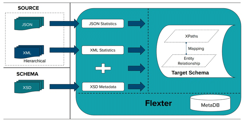
That’s exactly where Flexter Enterprise comes in. It takes everything you had to do manually and automates it end-to-end.
Pro tip
Flexter doesn’t just automate JSON to SQL; it also handles XML to SQL conversions end-to-end.
If you want to see how it ingests XML, maps it to relational tables, and handles schema evolution, check out articles like:
- XML to Database Converter – Tools, Tips, & XML to SQL Guide,
- How to Insert XML into SQL Tables (2026 Guide),
- XSD to Database Schema Guide – Create SQL Tables Easily.
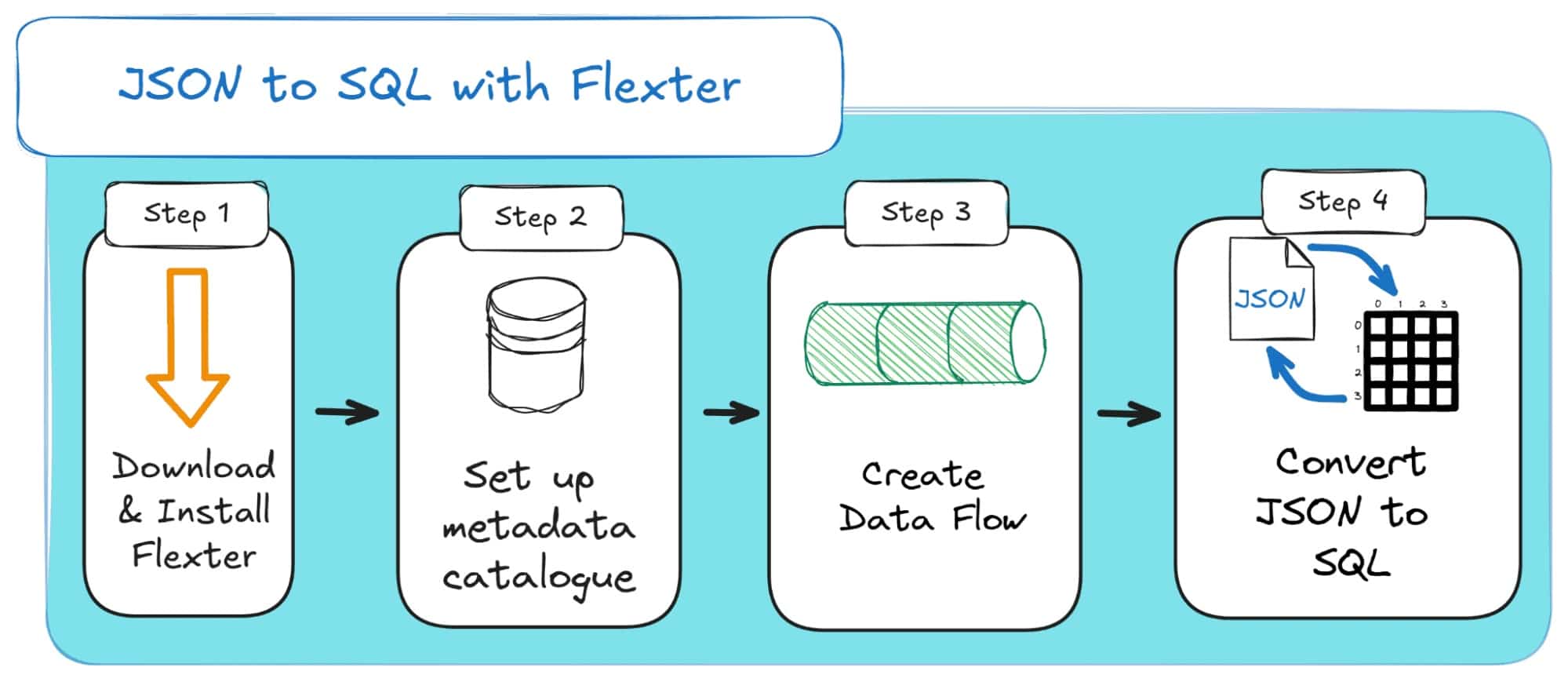
Here’s how the process works:
Step 1: Download & Install Flexter
First, you’ll need to install the Flexter binaries from the YUM/DNF repository.
You’ll need to contact Sonra to access the repository for free or request a 30-minute demo to get started.
To install the latest version, you can run:
|
1 |
$ sudo yum --enablerepo=sonra-flexter install xml2er xsd2er json2er merge2er flexchma flexter-ui |
This installs the JSON processing modules (json2er), schema management utilities, and the Flexter web interface.
Step 2: Configure the metadata catalogue
Before creating your first JSON project, set up the metadata database (metaDB).
This catalogue stores and manages all artefacts related to your automated conversions, including:
- Entity Relationship Diagrams (ERD),
- Source-to-target mappings,
- Automatically generated SQL DDL and DML scripts,
- Schema evolution history.
The detailed commands can be found in the detailed Flexter documentation.
Pro tip
Worried about designing the target SQL schema or mapping every JSON field to rows and columns?
You don’t have to be.
With an automated JSON to SQL solution like Flexter, those steps are handled for you: two simple commands, and the entire mapping and schema generation process is done automatically.
Check out Step 3 and Step 4 below ..!
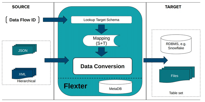
Step 3: Create a data flow
Next, define a data flow, the configuration that tells Flexter what to convert and where to store the results.
You can point Flexter to a single JSON file, a directory, or even a stream of incoming JSON messages.
Then Flexter will automatically capture parent-child relationships, array hierarchies, and data types before generating an optimised SQL table design for your target database.
As shown in our docs, you just need to run:
|
1 |
json2er -g1 /path/to/jsonfile.json |
Flexter stores the generated schema and metadata under a unique Data Flow ID, which you’ll use in the next step.
Here’s what data flow creation process with Flexter looks like:
Step 4: Convert JSON to SQL
Once your data flow is ready, execute the conversion by referencing the Data Flow ID.
Flexter reads and processes the JSON input, applies the inferred relational schema, and writes the output to your target system, whether that’s SQL Server, Snowflake, Redshift, or Delta tables on Databricks.
Here’s an example command, where you just specify parameters related to your system:
|
1 |
json2er -x<DataFlowID> -o jdbc:sqlserver://yourServer;databaseName=myDB -u myUser -p myPassword /path/to/jsonfile.json |
During the process, Flexter automatically creates all required SQL tables and generates the corresponding SQL insert statements.
It handles nested arrays, repeated elements, and evolving structures with no manual joins or key definitions required.
Here’s how the conversion process with Flexter looks like:
Pro tip
Flexter does not require or use JSON Schema definitions.
Instead, it infers the schema dynamically by analysing the data itself.
This makes it ideal for real-world use cases where JSON files evolve frequently or lack a defined schema, such as data streams, API payloads, or semi-structured logs.
Want to try JSON to SQL for FREE with Flexter?
Use our online converter, simply drag and drop your JSON file, and Flexter will instantly generate the SQL tables in Snowflake for you.
In this way, you’ll get a real taste of automated JSON to SQL conversion, including normalisation and automated documentation of your data model.
Try it now in the Flexter JSON to SQL Guide or the JSON to Snowflake Online Converter.
JSON to SQL: Best Practices and Patterns
Schema on Read vs. Schema on Write
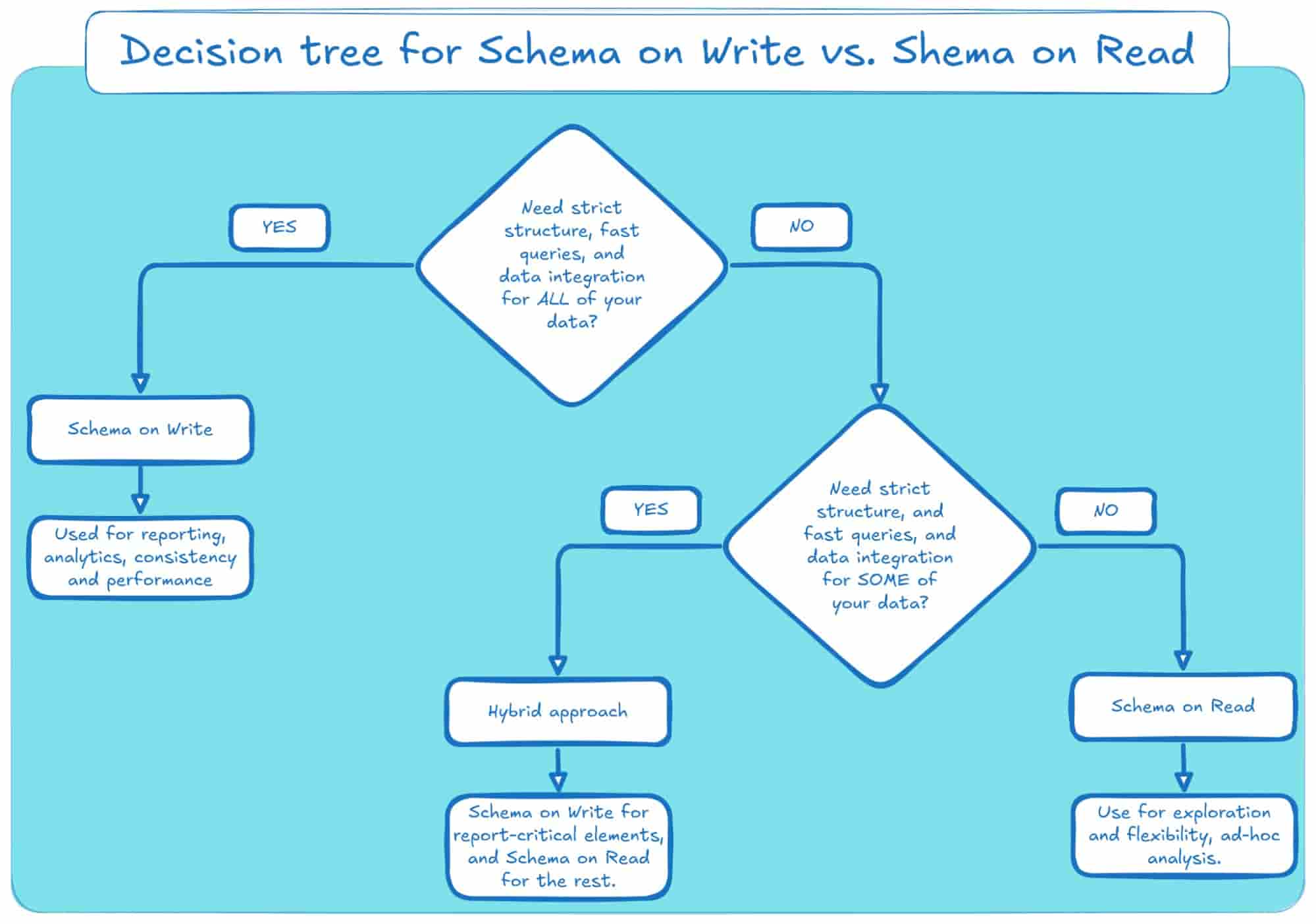
When working with JSON in databases, one of the first design decisions you’ll face is when to apply structure to your data.
Do you define your schema upfront, or do you load data first and worry about structure later?
This is the core difference between Schema on Write (SoW) and Schema on Read (SoR), and understanding this distinction is crucial before deciding how to manage your JSON data at scale.
TL;DR
This section covers crucial design strategies for successful JSON to SQL.
It compares Schema on Write (structure before loading) with Schema on Read (load raw data, structure later) and explains the benefits of a Hybrid Approach. It also details the critical choice between Normalisation (clean, related tables) and Flattening (one big table).
Be sure to check the Glossary at the end of this document to review definitions for any of these key terms.
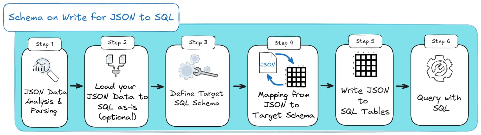
JSON to SQL with Schema on Write
With Schema on Write, you decide on the data structure before storing anything.
Think of it as building a house, you need blueprints before laying bricks.
This is the traditional database model: the schema enforces structure, data types, and relationships at write time.
Anything that doesn’t fit is rejected, which keeps data clean, predictable, and easy to query later.
Of course, it takes more effort upfront, you need to plan your schema, define keys, and handle schema evolution carefully, but the reward is consistent, query-ready data from the start.
Here’s the SOW process as a diagram:
Load JSON to SQL with Schema on Read
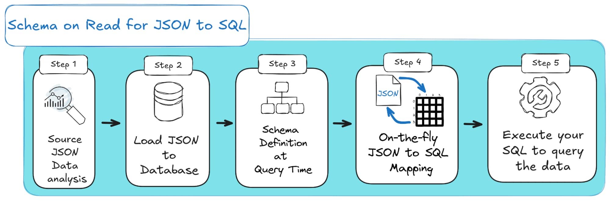
Schema on Read flips that idea completely. Instead of enforcing structure at ingestion, you store the data as-is, usually as raw JSON, and only apply structure when you query it.
Imagine dumping all your data into one big box and organizing it later, when you actually need it.
This makes loading data extremely fast and flexible, perfect for logs, event streams, and exploratory analysis where you don’t yet know what you’ll need.
The trade-off? Queries can become slower and more complex, since the database has to interpret structure on the fly.
Here’s how SOR looks as a diagram:
The Hybrid Approach for inserting JSON to SQL
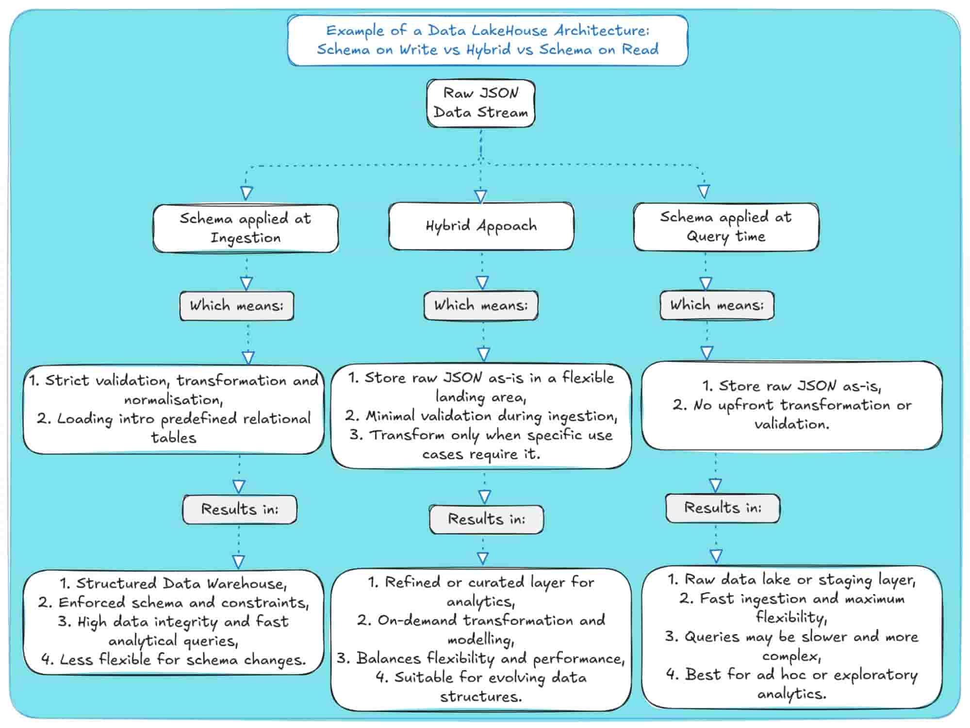
In reality, most modern data platforms, including Snowflake, Redshift, and Databricks, use a hybrid strategy.
You start by ingesting raw data quickly using a Schema-on-Read model, storing everything in its original form (for example, in Snowflake’s VARIANT column or a data lake’s raw zone).
Then, once specific use cases emerge, say, analytics or reporting, you transform and structure the data using Schema on Write.
This two-phase approach gives you the best of both worlds: agility upfront, consistency and performance later (when and where needed).
How it works:
- Ingest and Store Raw Data (SoR Phase): Load JSON directly into flexible storage without validation. Fast, simple, and keeps a single source of truth.
- Model for Specific Use Cases (SoW Phase): For production workloads, transform raw data into relational tables using ELT processes inside your database or warehouse.
Benefits of the Hybrid Model:
- Flexibility & Agility: Ingest now, model later.
- Performance & Integrity: Structured layers for critical workloads.
- Reduced Risk: Nothing gets rejected at ingest.
- Efficiency: Only transform what matters for your use cases.
If you visualize these three models side by side, the difference becomes clear.
Schema on Read offers maximum flexibility, Schema on Write provides structure and control, and the hybrid model bridges the two. capturing the best of both worlds.
Deciding between Schema on Read, Schema on Write and the Hybrid approach
To make this even clearer, here’s a quick comparison of how Schema on Write, Schema on Read, and the Hybrid approach differ in practice, from performance and agility to storage efficiency and governance.
|
Aspect |
Schema on Write (SoW) |
Schema on Read (SoR) |
Hybrid Approach |
|---|---|---|---|
|
When schema is applied |
Before data is stored (ingest time). |
When data is queried (access time). |
In stages: minimal schema on ingest, full schema on transformation/query. |
|
Ingestion speed |
Slower (validate/transform first). |
Faster (store raw data as-is). |
Fast: minimal validation on ingest, transformation happens later. |
|
Query performance |
Faster; data pre-structured and indexed. |
Slower; schema parsed/applied on the fly. |
Balanced: fast on curated/structured data, slower on raw data. |
|
Data quality & integrity |
High; strict validation prevents bad data. |
Variable; raw data can be messy/inconsistent. |
Managed: quality is enforced during transformation into curated layers. |
|
Flexibility & evolution |
Lower, schema changes are costly. |
Higher; easy to onboard new/variant data. |
High: raw zone accepts new formats easily; new models can be built on demand. |
|
Upfront modeling effort |
High; design schema, constraints, indexes. |
Lower, model later per use case. |
Moderate: model key use cases for curated layers, defer others. |
|
Risk at ingest |
Higher, non-conforming records may be rejected. |
Low: nearly all data lands; issues deferred. |
Low: most data lands in the raw zone; validation is deferred. |
|
Handling semi/unstructured data |
Harder; must fit a predefined schema. |
Easier: store first, interpret later. |
Ideal; stores raw data and applies structure as needed for use cases. |
|
Cost profile |
More engineering upfront; efficient queries. |
Cheaper to land data; more compute at query. |
Balanced: optimizes query compute by structuring high-value data. |
|
Time to value for new sources |
Longer—needs schema design/migration. |
Shorter, ingest immediately, model later. |
Short: data is available in the raw zone for exploration almost immediately |
|
Best for |
Regulated analytics, BI dashboards, stable workloads needing speed. |
Exploratory analytics, data science, varied/unknown schemas. |
Modern data platforms that need to balance BI, data science, and flexibility. |
|
Main drawbacks |
Inflexible, slower onboarding, schema migrations. |
Slower queries, potential data sprawl/quality debt. |
Increased complexity in managing multiple data zones and transformation logic. |
And if this is all still confusing, here’s a decision tree to help you reach a conclusion:
Denormalisation and Flattening versus Normalisation
When you’re moving JSON data into Snowflake, one of the first big decisions you’ll make is whether to flatten or normalise your source data.
That decision shapes how your semi-structured JSON ends up living in Snowflake’s relational world.
Get it wrong, and you’ll make life painful both when loading the data and when querying it later.
So let’s unpack what flattening and normalisation actually mean, and how each approach works in practice.
Pro tip
Flattening versus Normalisation is a challenge that will most likely come up when you decide to apply Schema on Write or the Hybrid approach.
With Schema on Read, you can just drop the JSON into a VARIANT column and call it a day.. though really, you’re just kicking the hard work down the road for the future you.
Normalisation: The Foundation of Relational Databases
What it is: Normalisation is about structuring your data to cut down on duplication and keep it consistent.
Instead of cramming everything into one wide table, you split it into smaller, related tables and connect them with primary and foreign keys.
The result is cleaner data, fewer errors, and a model that scales more gracefully as your dataset grows.
The goal with normalisation is simple: make sure every piece of information lives in just one place.
That way, you don’t run into messy update or delete errors, and your database stays clean and consistent.
Example: Normalised schema
Let’s consider that you and your team are working on a sales order database system.
If you were to store the data according to a normalised schema, then you would keep customer details in a dedicated customer table and orders in a separate orders table.
Both customers and orders point to a normalised geography hierarchy: cities -> states -> countries.
This avoids repeating country/state names on every row and keeps lookups clean.
Here’s how the ERD would look for such a schema:
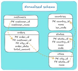
To provide the necessary connection between tables, a normalised schema utilises several Primary Keys (PK) and Foreign Keys (FK).
In our case, here’s how the tables connect through keys:
- customers.customer_id → orders.customer_id,
- orders.city_id → cities.city_id,
- cities.state_id → states.state_id,
- states.country_id → countries.country_id.
The trade-off? A highly normalised schema usually means more JOINs whenever you need to pull related data together through PKs and FKs.
On small datasets, that’s no big deal, but at scale, those joins can get expensive and slow down read-heavy workloads; exactly the kind you see in BI and analytics.
The other side: Flattening and Denormalisation
You’ll often hear flattening and denormalisation used almost interchangeably when talking about converting hierarchical data like JSON or XML into tables for a relational database.
However, they can have slightly distinct meanings in the broader field of data architecture.
Flattening involves converting a nested JSON structure into a single, flat table, sometimes referred to as a One Big Table (OBT).
You essentially unpack each branch of the source JSON file so that its contents appear as separate columns or rows. In Snowflake, the go-to tool for this job is the FLATTEN table function.
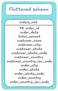
Example: Flattened schema
Take our first example of a sales order system: we store customer details, orders, and geographic information.
With flattening, all of that data is combined into a single table, known as the OBT.
The diagram below shows how the ERD looks for the flattened schema:
Denormalisation: This is the broader concept of intentionally introducing data redundancy to improve query performance. It’s the opposite of normalisation.
For example, you would usually apply denormalisation once you have converted your source JSON to a normalised structure, and we can then denormalise it for BI or analytics.
In the context of JSON, flattening always results in a denormalised table (as I showed you above).
The pre-joined, “wide” table (or OBT) created by flattening is a classic denormalised structure.
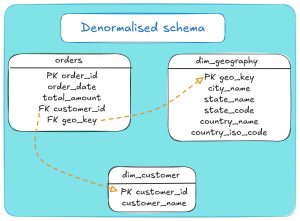
Example: Denormalising an initially normalised schema
In our sales order system example, you don’t always need to stick with a strictly normalised design, where customers and orders are stored in separate tables.
One option is to denormalise the normalised schema you initially created in Snowflake and consolidate much of it into a dimensional model.
Then your Snowflake schema (ERD) would look like this:
The dangers of flattening JSON with multiple branches
Flattening might look straightforward at first, but things get messy fast when your JSON has multiple independent branches.
For example, a branch typically represents a one-to-many relationship, where customers have multiple orders, orders contain multiple items, and payments utilise multiple methods.
If you just squash everything into one flat table, you risk duplicating data, losing context, or worse, breaking the very relationships that give your data meaning.
Next, I’ll show you an example of how flattening a JSON with multiple branches can get really complicated.
Example JSON Document
Let’s consider the following JSON document, which describes a university’s structure, including its faculties, departments, research groups, and administrative units.
|
1 2 3 4 5 6 7 8 9 10 11 12 13 14 15 16 17 18 19 20 21 22 23 24 25 26 27 28 29 30 31 32 33 34 35 36 37 38 39 40 41 42 43 44 45 46 47 48 49 50 51 52 53 54 55 56 57 |
{ "University": { "id": "TUD", "Faculty": { "id": "Engineering", "Department": [ { "id": "ComputerScience", "Course": [ "Introduction to Programming", "Algorithms and Data Structures" ] }, { "id": "ElectricalEngineering", "Course": [ "Circuit Analysis", "Electromagnetics", "Control Systems" ] } ], "ResearchGroup": [ { "id": "ArtificialIntelligence", "Project": [ "Machine Learning Advances", "Neural Network Optimization", "AI Ethics and Society" ] }, { "id": "Nanotechnology", "Project": [ "Nano-materials Engineering", "Quantum Computing" ] } ] }, "AdministrativeUnit": [ { "id": "Library", "Service": [ "Book Lending", "Research Assistance" ] }, { "id": "IT", "Service": [ "Campus Network", "Helpdesk" ] } ] } |
Identifying the Data Branches
Before you can decide how to model or convert your JSON, you first need to spot its branches.
Think of a branch as a full path that runs from the root of your JSON document down to a nested array of values.
Each of these paths highlights a different type of information, almost like separate storylines living inside the same file.
Let’s use the simple university JSON example I provided above.
Inside it, we can spot three distinct and meaningful branches:
- Courses Branch: University > Faculty > Department > Course
- Research Branch: University > Faculty > ResearchGroup > Project
- Services Branch: University > AdministrativeUnit > Service
Each branch represents a one-to-many relationship: one university, many courses; one research group, many projects; one administrative unit, many services.
Why does this matter? Because when you flatten and map your JSON into tables, each branch needs to be treated on its own.
Mix them up, and you’ll quickly end up with data duplication, NULL-flooded tables, or broken relationships.
The Danger: Flattening to a Single Table and the Cartesian Product
Yes, you can flatten the JSON university document I provided into an OBT.
But when you do, every item from the first branch gets combined with every item from the second, and then with every item from the third.
What you’ve just created is a Cartesian product. Huge, clumsy, and wrong.
This would happen because every course gets matched with every project and then repeated for every service.
I’ve made that mistake before, and trust me, it’s not a table you’ll ever want to query.
The JSON contains:
- 5 Courses (Introduction to Programming, Algorithms…, etc.)
- 5 Projects (Machine Learning Advances, Neural Network…, etc.)
- 4 Services (Book Lending, Research Assistance, etc.)
Attempting to create a single table would result in 5 x 5 x 4 = 100 rows.
Each row of the OBT is basically a blind date between a course, a project, and an administrative service.
A sample of the resulting rows would look like this:
|
University_id |
Faculty_id |
Department_id |
Course |
ResearchGroup_id |
Project |
AdminUnit_id |
Service |
|---|---|---|---|---|---|---|---|
|
TUD |
Engineering |
ComputerScience |
Introduction to Programming |
ArtificialIntelligence |
Machine Learning Advances |
Library |
Book Lending |
|
TUD |
Engineering |
ComputerScience |
Introduction to Programming |
ArtificialIntelligence |
Machine Learning Advances |
Library |
Research Assistance |
|
TUD |
Engineering |
ComputerScience |
Introduction to Programming |
ArtificialIntelligence |
Machine Learning Advances |
IT |
Campus Network |
|
… |
… |
… |
… |
… |
… |
… |
… |
|
TUD |
Engineering |
ComputerScience |
Introduction to Programming |
Nanotechnology |
Quantum Computing |
IT |
Helpdesk |
This single-table approach comes with three big risks:
- False and meaningless relationships: You end up creating links that never existed. Suddenly, “Introduction to Programming” looks tied to the “Quantum Computing” project and the “Helpdesk” service. You and I both know that makes zero sense; the only thing they share is being in the same university dataset.
- Massive multiplication and data bloat: One course shouldn’t expand to 20 rows simply because there are 5 projects and 4 services. But that’s exactly what happens. I’ve seen a single row explode into hundreds this way. Storage gets wasted, and good luck running even the simplest count without getting nonsense results.
- Broken integrity: The real relationships, like which courses belong to Computer Science, get buried under all the noise. What you’re left with is a table that looks structured but can’t be trusted for any serious analysis.
The Correct Approach: Flatten Each Branch Separately
The best approach is to normalise the JSON structure, but to keep things simple, you can also flatten each branch into its own table.
For example, consider the university JSON file.
Instead of forcing everything into one large and unwieldy OBT, you can break it down into separate tables that reflect the JSON’s branches: Courses, Research Projects, and Services.
Here’s how they would look:
Table 1: Courses (from the University > Faculty > Department > Course branch)
|
University_id |
Faculty_id |
Department_id |
Course |
|---|---|---|---|
|
TUD |
Engineering |
ComputerScience |
Introduction to Programming |
|
TUD |
Engineering |
ComputerScience |
Algorithms and Data Structures |
|
TUD |
Engineering |
ElectricalEngineering |
Circuit Analysis |
|
TUD |
Engineering |
ElectricalEngineering |
Electromagnetics |
|
TUD |
Engineering |
ElectricalEngineering |
Control Systems |
Table 2: Projects (from the University > Faculty > ResearchGroup > Project branch)
|
University_id |
Faculty_id |
ResearchGroup_id |
Project |
|---|---|---|---|
|
TUD |
Engineering |
ArtificialIntelligence |
Machine Learning Advances |
|
TUD |
Engineering |
ArtificialIntelligence |
Neural Network Optimization |
|
TUD |
Engineering |
ArtificialIntelligence |
AI Ethics and Society |
|
TUD |
Engineering |
Nanotechnology |
Nano-materials Engineering |
|
TUD |
Engineering |
Nanotechnology |
Quantum Computing |
Table 3: Services (from the University > AdministrativeUnit > Service branch)
|
University_id |
AdministrativeUnit_id |
Service |
|---|---|---|
|
TUD |
Library |
Book Lending |
|
TUD |
Library |
Research Assistance |
|
TUD |
IT |
Campus Network |
|
TUD |
IT |
Helpdesk |
With the multi-table setup, you finally get a structure that mirrors the original data, skips the duplication mess, and, most importantly, keeps the real relationships intact so your analysis actually makes sense.
Pro tip
If you’ve worked with XML before, this should feel familiar.
Multi-level flattening in JSON is equivalent to converting multi-branch XML into SQL tables.
Each branch must be expanded manually step by step (using a LATERAL join with FLATTEN), and every join carries the parent context forward.
The same warning applies too, flatten too aggressively, and you risk cartesian blow-ups with duplicate or redundant rows.
Normalisation or flattening? Choosing the right approach
It is important to distinguish between the role of normalisation and flattening/denormalisation in the data lifecycle.
When ingesting JSON into a relational system, such as Snowflake, the preferred method should always be normalisation. Only for very simple schemas, it might be OK to denormalise.
A normalised schema provides a process-neutral representation of the data: it avoids redundancy, preserves integrity, and serves as a flexible foundation that can support diverse downstream use cases.
Flattening, or denormalising your source JSON data in any shape or form, creates redundant and repeated values in your target schema database.
Inserting data in Snowflake with flattening should never be your goal.
It may be an easy approach to understand and implement, but most likely, you will pay for that in engineering time (reworking, renormalisation) as well as Snowflake credits in the long term.
With that being said, flattening or denormalisation can be a deliberate optimisation step applied later on to your database, typically for building reports, dashboards or analytical models.
In these scenarios, redundancy can be introduced intentionally to simplify queries and reduce join costs, resulting in structures such as dimensional models (for business intelligence) or OBT (for machine learning).
The key principle is to normalise first in your integration layer, denormalise later in your access layer.
However, you need to remember: once data has been denormalised, it is difficult to reconstruct a normalised schema, whereas normalised data remains adaptable to any context.
Pro tip
Flattening is just one flavour of denormalisation.
In the broader context, denormalisation may involve any shortcut you take to make reads faster, such as:
- materialising joins into a single table,
- duplicating lookup fields (e.g., department_name on a fact table),
- precomputing aggregates, or,
- rolling up hierarchies into a single dimension.
In other words, flattening is always denormalisation, but denormalisation is not always flattening; it’s any redundancy you introduce to speed up a specific access path.
Practical Example on Normalisation vs. Flattening vs. Denormalisation
The best way to illustrate the differences between the three approaches is with a hands-on example.
Next, I’ll provide a hands-on example that you can follow to convert a simple JSON test case using the three methods.
Normalising JSON in SQL
If you use Flexter Online, you can easily drag and drop this JSON file, and the online tool will normalise your source data and insert it into a Snowflake instance in a matter of seconds (or minutes).
If you access the data (as I show in my step-by-step guide) you’ll see that the original JSON is converted into five new tables that include your data (six, including the ROOT table with your metadata).
Here’s how it looks on Snowflake:
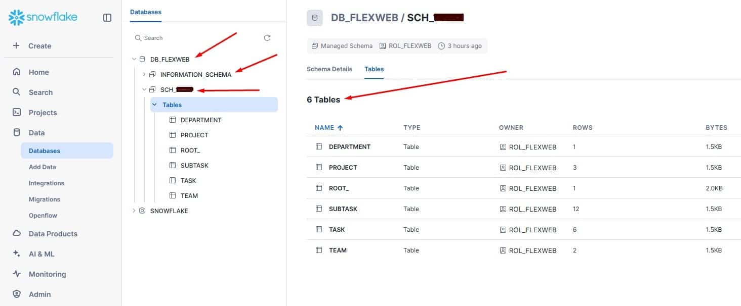
If you inspect the contents of the generated tables, you’ll see that the conversion tool automatically normalises your data into separate tables and sets up the primary and foreign keys to define the relationships between them.
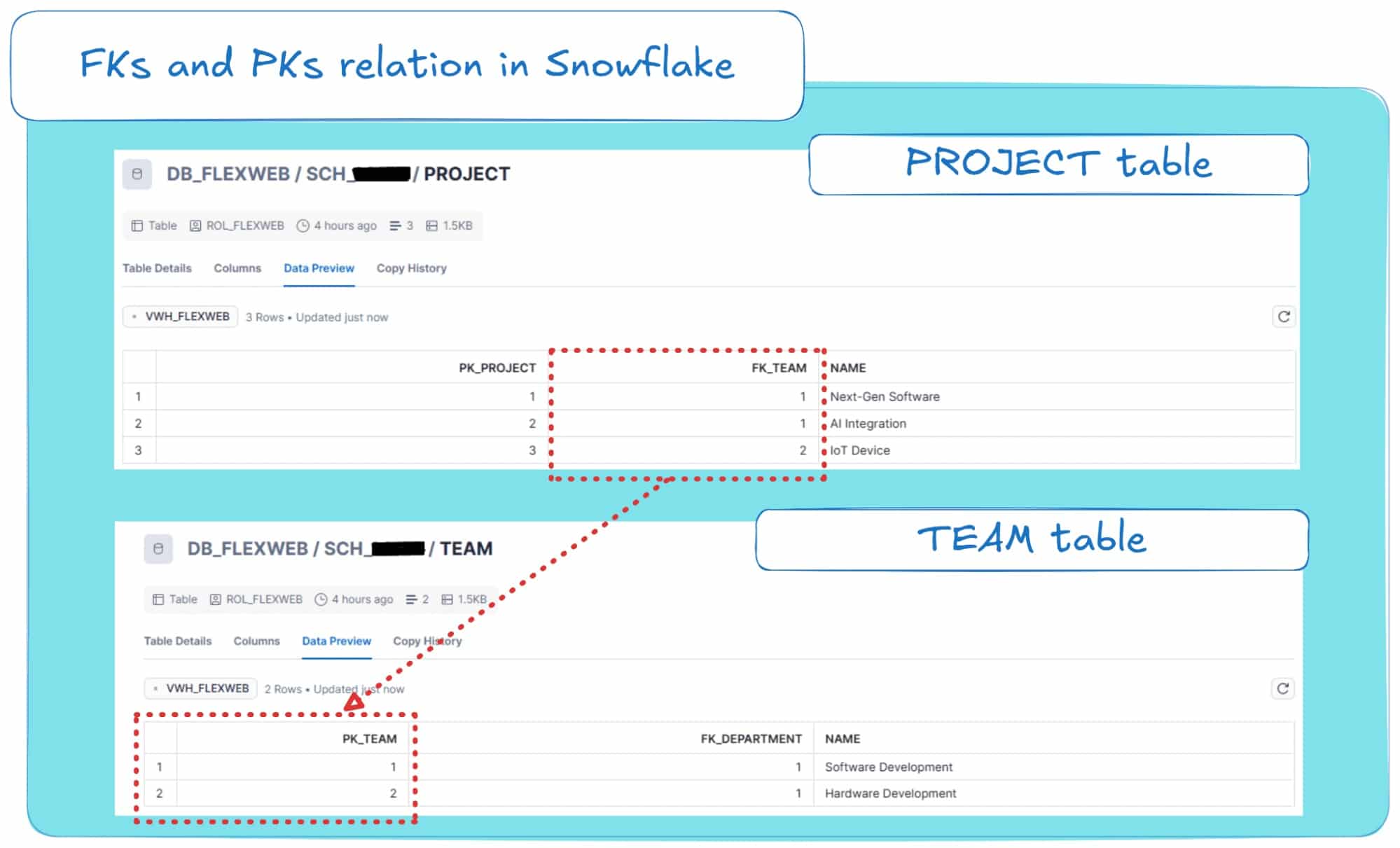
Below, I show you how the PROJECT table (which includes all projects from the source JSON) and the TEAM table (which includes teams) connect using primary and foreign keys.
Flattening your source JSON into SQL tables
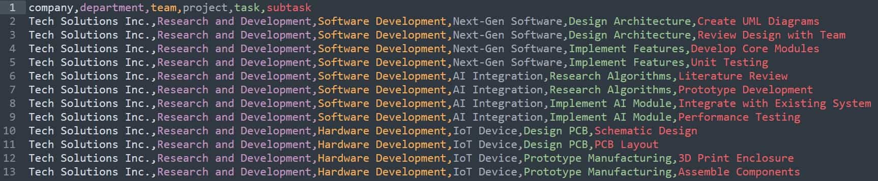
Flattening your source JSON into a One Big Table (OBT) essentially involves a full unwind of the hierarchy: explode every nested array/object, then propagate the parent attributes down so that each row carries its full context.
It’s a straightforward transformation, so plenty of off-the-shelf tools can take raw JSON and materialise an OBT that looks like this:
Normalisation avoids this monstrous OBT by factoring entities into separate tables and linking them with keys, so growth is closer to the sum of parts rather than their product.
You join only what you need at query time, preserving flexibility without paying the OBT tax everywhere.
Denormalising an initially normalised schema
Denormalisation takes a clean, normalised schema and reshapes it into wider tables by materialising common join paths.
In practice, this really helps with BI dashboards and reporting (think star or snowflake schemas) as well as with ML use cases, where a single OBT enables much quicker feature access.
I will include a small practical denormalisation example here, based on the normalised schema that Flexter Online derived for our source JSON file.
Starting from a normalised schema with separate Company, Team, Project, Task, and Subtask tables, we can denormalise by combining Task and Subtask into a fact table and creating Project and Department dimension tables.
This yields a schema where each fact row represents a subtask (or a task if no subtasks exist), linked by surrogate keys to descriptive project and department dimensions.
The result is a star schema with three tables:
- fact_task_work (one row per subtask)
- dim_project (project and team details)
- dim_department (company and department details)
This design reduces the number of joins needed for reporting, since analysts can directly slice facts by project or department attributes, while still keeping dimensions relatively compact and descriptive.
The tables are shown below:
Table dim_department:
Table dim_project:
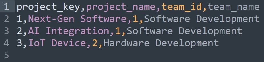
And the table fact_task_work:
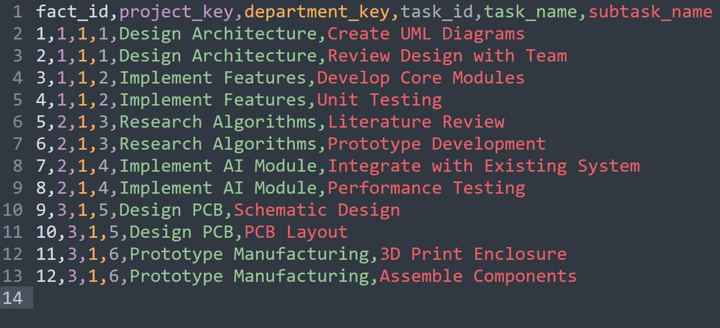
Introducing a fact table that materialises the join of TASK and SUBTASK yields a schema that breaks higher normal forms and introduces redundancy not implied by keys alone.
Once you denormalise your source JSON data or relational schema, reversing back to a fully normalised design is hard in practice, because denormalised layouts aren’t process-neutral: they encode assumptions about how the data will be read.
The upside is clear: simpler queries, predictable performance, and fewer moving parts at read time.
The downside is equally important: intentional redundancy, more frequent updates, and reduced flexibility for answering new questions.
That’s why the common pattern is to keep data normalised for ingestion and stewardship, and then denormalise selectively into OBTs that align with the specific read paths you need to support.
Comparison table
And here’s a table to sum it up:
|
Approach |
What is it |
Pros |
Cons |
|---|---|---|---|
|
Normalisation |
Splitting data into multiple related tables (using primary/foreign keys) to minimise redundancy and preserve integrity. |
Clean design, no redundancy, consistent updates. |
Requires joins to reconstruct full records; queries can be slower for analytics. |
|
Flattening |
Converting nested JSON into a single, flat table. Arrays and objects are unpacked into rows/columns. |
Simple to query for very specific cases and small datasets, where you may produce One Big Table (OBT). |
Data redundancy, larger tables, and harder to maintain consistency for most real-world JSON (deeply nested files, multiple branches). |
|
Denormalisation |
Introducing redundancy intentionally to make querying faster. Flattening produces a denormalised structure. |
Use cases such as BI, dashboards and analytics tools can query a wide table directly, without joins. |
Wastes storage, harder to update consistently (risk of anomalies). |
FAQ
1. What’s the difference between loading JSON into a database and converting it?
Loading JSON means you are simply storing the data as-is in its raw, semi-structured form.
Converting, on the other hand, is the process to convert JSON to a SQL database.
This involves transforming the semi-structured data into a structured, relational model with defined tables, columns, keys, and data types, which is essential for making it optimized for analytics and integration.
2. What are the main ways to ingest JSON data into a database?
There are four primary methods for ingesting JSON, each offering a different balance of speed (latency) and volume (throughput) before you convert JSON into SQL table structures:
- External Tables: Allows you to query JSON in SQL directly from object storage without loading it, which is ideal for initial exploration.
- Batch Loading: Ingests large volumes of JSON data periodically using bulk commands like COPY INTO. This method prioritizes high throughput over low latency, making it a common step in ETL JSON to SQL pipelines.
- Streaming Ingestion: Continuously pushes JSON data from sources like message queues for near-real-time availability.
- API or Application Inserts: Writes JSON records directly from an application, common for transactional systems that require immediate consistency and a direct JSON to SQL insert.
If you want to take a look at a comparison table on those four options, click here.
3. What are my options for storing JSON in a database?
When deciding how to store JSON in a SQL database, you have two main choices:
- Textual Storage: The JSON is stored as a simple text string (TEXT, VARCHAR, etc.). This preserves the exact original format but is slow to query because the database must parse JSON on every request.
- Binary Storage: This is a more modern approach where the database uses a native JSON data type SQL supports, like jsonb or VARIANT. The JSON is parsed upon ingestion and stored in an optimized binary format, which is much faster for querying JSON in SQL and allows for advanced indexing.
4. What’s the difference between “schema on write” and “schema on read”?
The difference lies in when you apply a structure to your data during the JSON to SQL process:
- Schema on Write (SoW) is the traditional database approach where you define a strict schema (tables, columns, data types) before writing the data. SoW ensures fast query performance.
- Schema on Read (SoR) involves storing the raw, unstructured data first and only applying a schema when you read or query it. This is faster for ingestion and more flexible, especially when the source JSON schema changes frequently.
5. When should I use a SoW and SoR hybrid schema approach?
A hybrid approach is ideal for modern data platforms because it offers the best of both worlds for working with JSON in SQL.
You start by ingesting raw JSON quickly using a schema on read model into a flexible storage layer. Later, for specific use cases like BI reporting, you transform that raw data into structured, query-optimized relational tables using a schema on write model.
This balances agility with performance and integrity.
6. What’s the difference between normalizing and flattening JSON?
When you convert JSON to a SQL table, you must decide how to handle its structure:
- Normalisation is the process of breaking down a nested JSON to a SQL table structure by creating multiple smaller, related tables connected with primary and foreign keys. The goal is to reduce data redundancy and improve data integrity.
- Flattening is a form of denormalization that converts a nested JSON structure into a single, wide JSON table, often called a One Big Table (OBT). Every nested element is unpacked to become a column or row in this single table.
7. Why is flattening a JSON file dangerous sometimes (e.g. JSON with multiple branches)?
If your JSON has multiple independent arrays (branches), forcing them into one flat table will create a Cartesian product. This incorrectly multiplies the data, creating massive redundancy and false relationships between unrelated items. When you need to generate a table from JSON data with multiple branches, the correct approach is to flatten each branch into its own separate table to maintain data integrity.
8. Best practises: Should I normalize or flatten my JSON data first?
For initial data integration, the best practice is to normalise first. This creates a clean, flexible, and process-neutral representation of your data in the database that avoids redundancy. Flattening and denormalization should be used as a later, deliberate optimization step for specific use cases (like creating a single datatable from JSON for a BI dashboard) where query speed is more important than data redundancy.
9. What is Flexter?
Flexter is an enterprise-grade, no-code JSON to SQL converter that automates the conversion of large and complex JSON and XML files into a relational format. It simplifies the process of making semi-structured data available for analytics by automatically discovering the JSON to SQL schema, mapping the data, and generating the relational output without manual coding.
10. What are the key benefits of using an automated tool like Flexter?
The main benefits of using Flexter for your JSON to database projects are:
- Automation: It automates the entire conversion process, eliminating the need for time-consuming manual coding to parse JSON in SQL.
- Scalability: Built on Apache Spark, it is designed to handle massive datasets and millions of files efficiently.
- Speed: It drastically reduces project timelines for data conversion tasks.
- Cost Savings: By automating manual work, it reduces development effort and the need for specialized expertise.
You can find a detailed list of Flexter’s differentiators to other converter solutions at my other blog post.
Glossary
|
Term |
Explanation |
|---|---|
|
JSON (JavaScript Object Notation) | A data format used to power API integrations, event streams, and user data. It is a semi-structured data format. |
|
One Big Table (OBT) |
A single, flat, wide table that results from flattening a nested JSON structure. It is a classic denormalized structure often used for machine learning or specific BI use cases. |
|
Cartesian Product | An undesirable outcome of improperly flattening JSON with multiple independent branches into one table. It occurs when every item from one branch is combined with every item from all other branches (e.g., 5 courses x 5 projects x 4 services = 100 rows) , resulting in massive data bloat and false, meaningless relationships. |
|
Flattening |
A data modeling approach that converts a nested JSON structure into a single, flat table, often called a One Big Table (OBT). |
|
Normalisation |
A data modeling approach that structures data to minimize duplication and maintain consistency. It involves splitting data into smaller, related tables that are connected using primary and foreign keys. |
|
Denormalisation |
The broad concept of intentionally introducing data redundancy to a database schema to improve query performance. It is the opposite of normalisation. Flattening is considered a form of denormalization. |
|
Hybrid Approach (Schema) |
A strategy that combines Schema on Read and Schema on Write, as presented in my detailed blog post sub-section. |
|
Schema on Read (SoR) |
A data management approach where data is stored as-is in its raw form (like JSON) without enforcing a structure at the time of ingestion. The schema is applied only when the data is queried or read. |
|
Schema on Write (SoW) |
The traditional database model where a strict data structure (schema, data types, relationships) is defined before any data is stored or written. |
|
SQL/JSON Path Language | An ISO standard (ISO/IEC 9075) that defines a consistent syntax for navigating, extracting , and filtering data from within JSON documents using SQL. |
|
Throughput | One of two critical dimensions for data ingestion. It is defined as the amount of data processed per unit of time. |
|
Latency | One of two critical dimensions for data ingestion. It is defined as the delay between when data is generated and when it becomes available for querying. |
|
Streaming Ingestion |
One of the four primary ingestion paradigms. This is a low-latency approach where JSON data is continuously captured and delivered as events occur, typically flowing from sources like APIs or IoT sensors through message queues into the database. |
|
External Tables |
One of the four primary ingestion paradigms. This method allows you to query JSON files directly from object storage (like S3, Azure Blob Storage, or GCS) without physically ingesting the data into the database. |
|
Batch Loading |
One of the four primary ingestion paradigms. This is a high-throughput method where JSON data is collected and then ingested periodically in large, bulk batches, using commands like COPY, bq load, or COPY INTO. It optimizes for throughput over latency. |
|
Applications Programming Interface (API) | A set of rules that allows different software applications to communicate and exchange data. APIs are a common source of JSON data (like payloads or event streams) and are also used by applications to write data directly into databases. |
|
API or Aplication Inserts |
One of the four primary ingestion paradigms. This method involves an application or microservice writing JSON directly into the database, often one record at a time. It is suited for transactional workloads and focuses on immediacy and control rather than bulk throughput. |
|
Textual JSON Storage |
A simple storage method where the JSON data is saved as-is in a plain text column, such as TEXT, CLOB, or VARCHAR. |
|
Binary JSON Storage |
A modern storage approach where JSON is parsed once upon ingestion and stored in a tree-like structure. |
Uli Bethke
Uli has been rocking the data world since 2001. As the Co-founder of Sonra, the data liberation company, he’s on a mission to set data free. Uli doesn’t just talk the talk—he writes the books, leads the communities, and takes the stage as a conference speaker.
Any questions or comments for Uli? Connect with him on LinkedIn.
Follow Uli Bethke: