Sampling in Snowflake. Approximate Query Processing for fast Data Visualisation

Introduction

Making decisions can be defined as a process to achieve a desirable result by gathering and comparing all available information.
The ideal situation would be to have all the necessary data (quantitatively and qualitatively), all the necessary time and all the necessary resources (processing power, including brain power) to take the best decision.
In reality, however, we usually don’t have all the required technical resources, the necessary time and the required data to make the best decision. And this is still true in the era of big data.
Although we have seen an exponential growth of raw compute power thanks to Moore’s law we also see an exponential growth in data volumes. The growth rate for data volumes seems to be even greater than the one for processing power. (See for example The Moore’s Law of Big Data). We still can’t have our cake and eat it 🙁
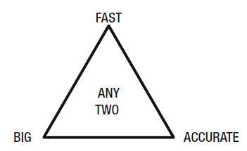
If we want a fast response, we either reduce the size of the data or the accuracy of the result. If we want accurate results, we need to compromise on time or data volumes.

In other words for data processing we can have fast and big but not accurate, fast and accurate but not big, or big and accurate but not fast, which is neatly depicted in the diagram below.

Approximate Query Processing.

Approximate Query Processing (AQP) is a data querying method to provide approximate answers to queries at a fraction of the usual cost – bot in terms of time and processing resource: big data and fast but not entirely accurate.
How is it done? We can use sampling techniques or mathematical algorithms that can produce accurate results within an acceptable error margin.
But, when is the use of AQP acceptable? Certainly not for Executive Financial Reporting or Auditing.
However, the main objective for data analytics is not generating some boring financial report, it is rather the reduction of uncertainty in the decision making process. This is accurately captured in the term Decision Support System, which in my opinion is a much better term for working with data than say data warehousing, big data or data lake. DSS reminds us that we are not doing data analytics just for the sake of it. Approximate queries certainly fit the bill here. They reduce uncertainty trading off speed versus accuracy, perfectly acceptable in the vast majority of decision making use cases.
Let’s have a look at an example. We will use the wonderful sampling features of the Snowflake database to illustrate the point.

Making perfect decisions with imperfect answers. Plotting data-points on a Map

Considering that

1. There are a finite number of pixels on your screen, so beyond a certain number of points, there is no difference.
2. The human eye cannot notice any visual difference if it is smaller than a certain threshold.
3. There is a lot of redundancy in most real-world data-sets, which means a small sample of the entire data-set might lead to the same plot when visualized.

It’s similar to viewing pictures. You can take that great shot with a professional 30 Megapixel camera. Viewing it on your tablet, you barely see a difference if it had been taken with a compact camera. At least as long as you don’t try to zoom in deeply, which you’d probably only do in case you found something interesting to drill into. So, to decide if your data is worth to be looked at in more detail you don’t need to see each and every data point.
The same approach can be used with plotting points on a map (screen), using a sample instead of the whole data set.

Sampling on Snowflake.

Snowflake sampling is done by a SQL select query with the following Syntax:

There are two sampling methods to use, identified by samplingMethod  ( <p> ):

• BERNOULLI or ROW: this is the simplest way of sampling, where Snowflake selects each row of the FROM table with <p>/100 probability. the resulting sample size is approximately of <p> /100 * number of rows on the FROM expression.
• SYSTEM or BLOCK: in this case the sample is formed of randomly selected blocks of data rows forming the micro-partitions of the FROM table, each partition chosen with a <p>/100 probability.

The REPEATABLE | SEED parameter when specified generates a Deterministic sample, ie. generating different samples with the same <seed>  AND <probability> from the same table, the samples will be the same, as long as the table hasn’t been updated.
It’s important to note that:

• You cannot use SYSTEM/BLOCK nor SEED when sampling from Views or sub-queries
• Sampling from a Copy Table may not produce the same sample as the original for same probability and seed values
• Sampling without a seed and/or using Block sampling is usually faster

Which option should you use, ROW or SYSTEM? : according to the Snowflake documentation, SYSTEM sampling is more effective – in terms of processing time – with bigger data sets, but more biased with smaller data sets, so without further evaluation this would be the basic rule: use SYSTEM/BLOCK for higher volumes of data rows and ROW/BERNOULLI for smaller tables. I suspect the using of particular sets of table partitioning keys, if any, might have some influence too.

Our Example

With the use of Tableau Public, a public version of the great Visual Data Analysis Tool, we will plot several points on the map of the United States using a data set available at https://public.tableau.com/s/resources, particularly the voting records of the 113th US Congress.
It’s an Excel file which has two sheets, that we transformed into csv files,
US_113thCongress-Info.csv – containing the different Bills information, including sponsor party and State, that we loaded as US_BILL.
and
US_113thCongress-Votes.csv – containing the voting sessions, their results and number of votes by Party, that we loaded as US_BILL_VOTE.
The idea here is to generate a reasonable big number of records with geographic coordinates to be ploted on a map.
To achieve this, we merged the tables above with another table we downloaded from US Cities Database | Simplemaps.com , uscitiesv1.4.csv, a text file with all US Cities with geographic coordinates (points).
The number of records (data points per table/join)

TABLE_NAME	ROW_COUNT
US_BILL	286
US_BILL_VOTE	4410
US_CITY	36650
JOIN	4,728,604

As a result we have a table with 4M records and a lot of redundant points spread over the US map. Since the goal is to sample and produce an accurate coverage of the map, it’s good for our purposes.
To evaluate the sampling accuracy we selected 3 variables: Sponsor Party (of the Bill), Quantity of (distinct) Bills and distinct Counties covered by the sample.
As Tableau Public, doesn’t allow ODBC or JDBC connections, we exported the samples to text files and connected Tableau to them.

Samples

We produced 4 data sets:

• Full data – the full table (US_BILL_VOTE_GEO) resulted from our join
• Substract – the exported table had been downloaded in 13 text files and we selected every 3^rd of them to create a non-random sample
• Sample 1 using Block Sample (10%) – SELECT * FROM BILL_VOTE_GEO SAMPLE SYSTEM(10)
• Sample 2 using Row Sample (10%) – SELECT * FROM BILL_VOTE_GEO SAMPLE ROW(10)

Results

We produced two sets of graphics, one for each of the main Parties (Democrats and Republicans). Since the sample should represent the distribution of points for each Party in a similar pattern to the full data, we will evaluate the graphical output for each of these parties separately as an evidence of the samples accuracy.

Democrats – Full Dataset – 26 States with 54 from democrats sponsored bills	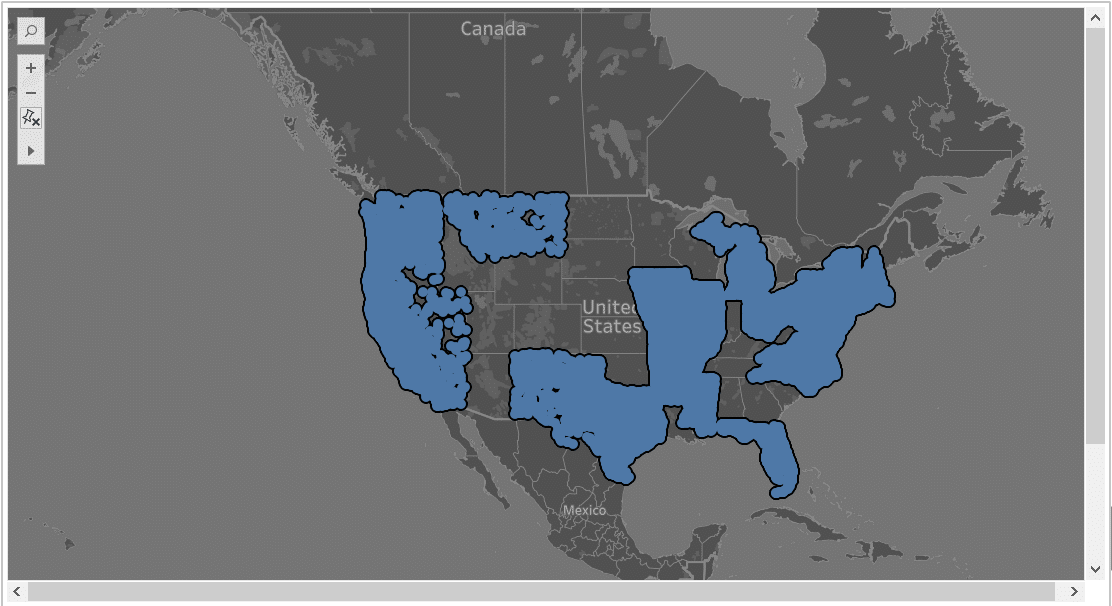Democrats – Substract Dataset – 12 States with 26 from democrats sponsored bills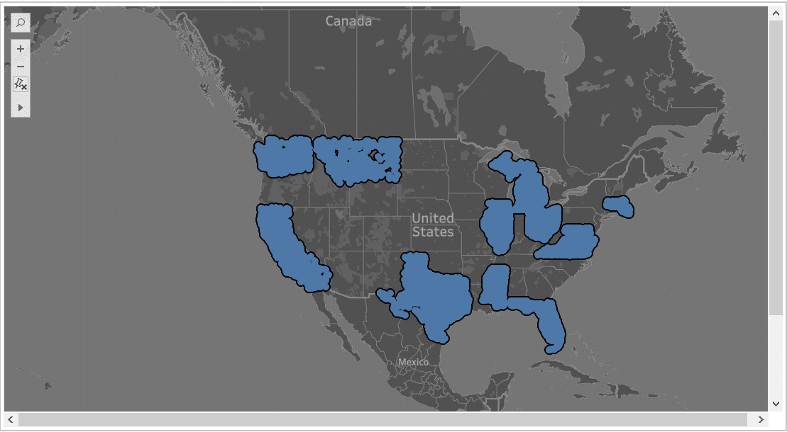
Democrats – Random BLOCK Sample – 22 States with 29 from democrat sponsored bills	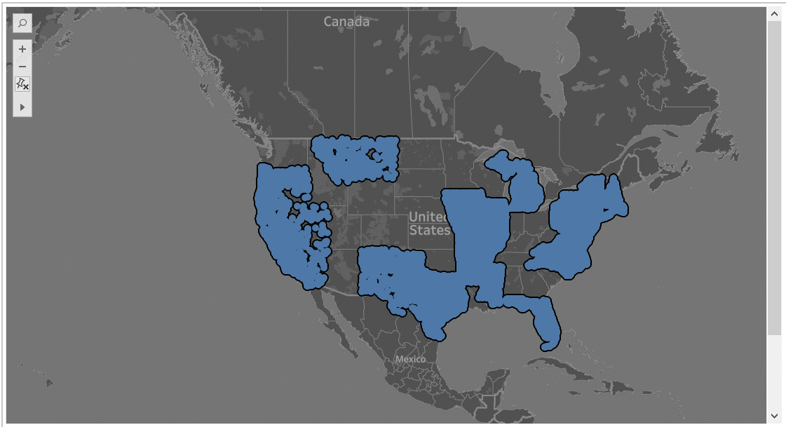Democrats – Random ROW Sample– 26 States with 54 from democrats sponsored bills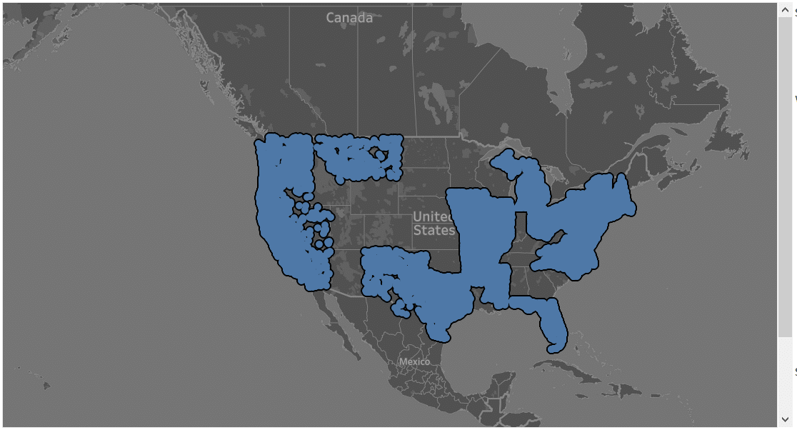

Republicans – Full Dataset – 34 States with 231 from Republicans sponsored bills	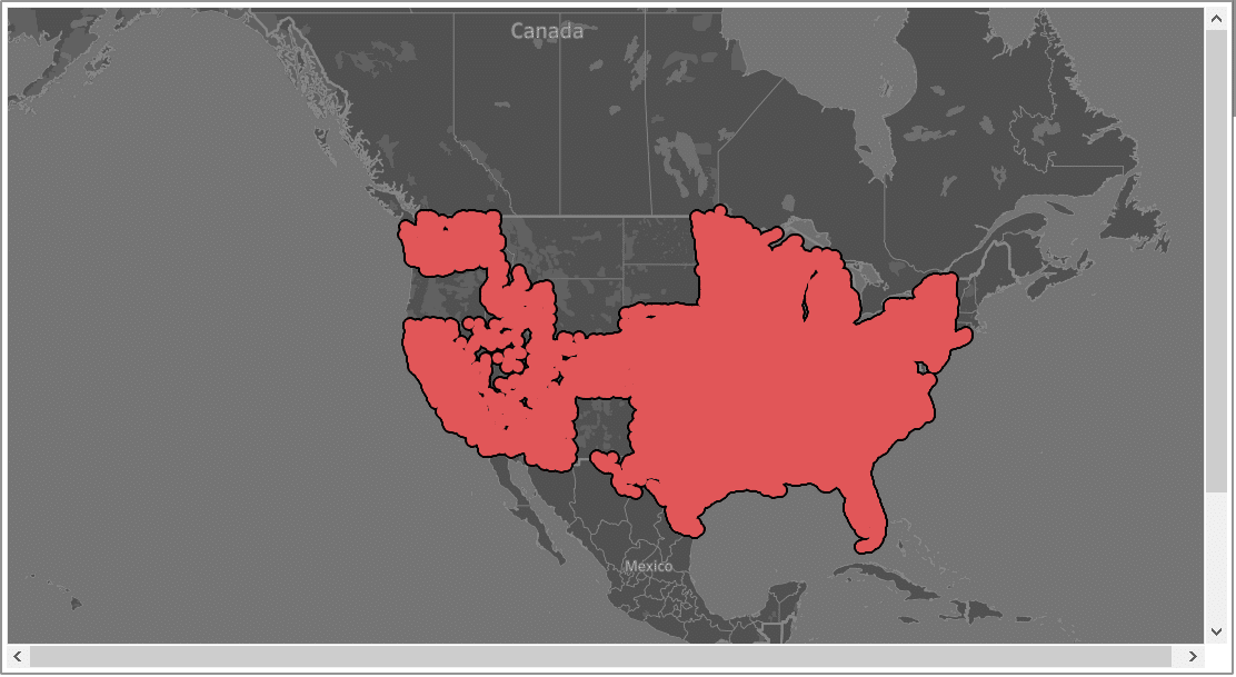Republicans – Substract Dataset – 23 States with 170 from Republicans sponsored bills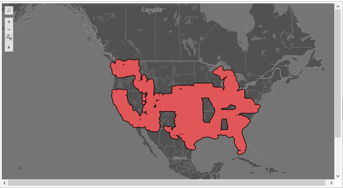
Republicans – Random BLOCK Sample – 31 States with 154 from Republicans sponsored bills	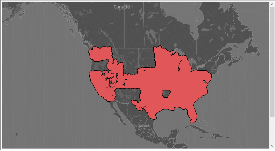Republicans – Random ROW Sample– 34 States with 231 from Republicans sponsored bills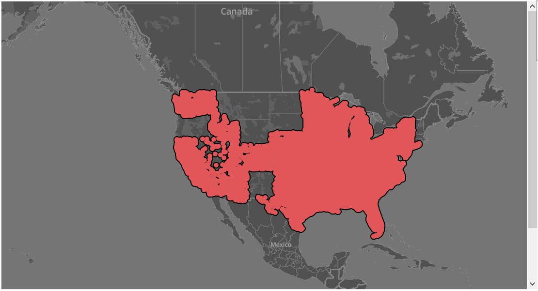

As we can see, the maps for both Republicans and Democrats data-points of the Random Samples (bottom rows) are remarkably similar to the full Dataset (top-left). They are different to the non-random sample (strata) that lacks the accuracy.
Between the random samples, the Row (Bernoulli) random sample appears to be a little more accurate than the block random sample.
The table below express the percentage in number of records for each Party in each analysed set of data ordered by accuracy from left to right.

Sponsor Party	Full Dataset	Random ROW	Random BLOCK	Strata (Not random subset)
R	90.74%	90.70%	89.36%	95.62%
D	9.17%	9.20%	10.60%	4.29%
I (Independent)	0.05%	0.05%	–	–
Null (No Bill)	0.05%	0.05%	0.04%	0.08%

As it can be seen from the table above, there are data-points not covered in our graphics, related to bills sponsored by Independents (1) and States (5) with no Bills sponsored, representing only 0.1% of the data, and this data was better captured by the Random Row sample.

Conclusions

The main purpose of data analytics is to support business decision making. This is achieved by reducing the amount of uncertainty. Reducing the amount of uncertainty does not require perfectly accurate data, at least for most decisions. Forward thinking database vendors such as Snowflake reflect this reality by providing approximate query features to data analysts.
Here are some other takeaways:

• Smart trumps big in many cases. Often you don’t need the smartest and latest distributed big data framework to improve your business decisions and make a difference to your bottom line.
• From this case we could see that random sampling can be used to get actionable analytical results, in particular with visual data (Graphics)
• Snowflake uses random samples, either by randomly selecting rows or randomly selecting blocks of data (based on the micropartion schema adopted by Snowflake). These can be used to reduce the data volume to achieve actionable results with low loss of accuracy. This accuracy will still depend on the complexity of the required analysis and the kind of sampling adopted.
• As stated by the Snowflake documentation, Block sampling can be more biased for smaller sets of data. In our case with 4 million records the random row sample was more accurate.
• It was much more performant and quicker to build our dashboard with the sampling queries. This can make an important difference Our experience on building and shaping the dashboard showed that a reduced set of data-poins had made a difference in terms of performance, that can be important in ad-hoc analysis.

Enjoyed this post? Have a look at the other posts on our blog.
Contact us for Snowflake professional services.
We created the content in partnership with Snowflake.