Introduction to Window Functions on Redshift

Use Flexter to turn XML and JSON into Valuable Insights
- 100% Automation
- 0% Coding
Benefits of Window Functions
Window functions on Redshift provide new scope for traditional aggregate functions and make complex aggregations faster to perform and simpler to write. Window functions also allow the SQL developer to look across rows and perform inter-row calculations.
The main benefits are:
- Possibility of summarization over dynamically shifting view (sequence of rows called window), e.g. when we want to get an average of last five values for each day. The window is highly customizable, as we will see later.
- Summarization is produced for each qualifying row, not a group, therefore, we can include any other attribute in the output, which was not possible with aggregate functions unless we group over it.
- We can compute values over multiple aggregations in one SELECT clause.
The alternative to window functions are self joins or correlated subqueries. However, window functions are more simple to read and perform better. Let’s compare the two. We keep some values together with a date and would like to get the original table enriched with the sum of values over all dates. Without window functions, a self join or in this particular scenario a cross join is the obvious solution:
SELECT
  date,
  value,
  sum_table.sum_value
FROM
  values,
  ( SELECT sum(value) AS sum_value FROM values ) AS sum_table;
The solution using window functions does not need to join tables:
SELECT
  date,
  value,
  sum(value) OVER ()
FROM values;
The latter solution is also faster. It just needs one sequential scan of the table values. The self join requires two scans.
Most relational databases such as Oracle, MS SQL Server, PostgreSQL and Redshift support window functions. MySQL does not. All of the following queries have been tested with PostgeSQL and Redshift.
Syntax
We may use window functions only in the SELECT list or ORDER BY clause.
window_function(expression) OVER ( [ PARTITION BY expression]
[ ORDER BY expression ] )
We need to specify both window and function. The function will be applied to the window. With the PARTITION BY clause we define a window or group of rows to perform an aggregation over. We can think of it as a GROUP BY clause equivalent, though the groups will not be distinct in the result set. ORDER BY defines the order of rows in a window. The expression will be passed over to the function in the same order.
We can apply window functions to all aggregate functions, such as:
- sum(expression) sum of expression across all input values
- avg(expression) arithmetic mean of all input values
- count(expression) number of input rows for which the expression is not null
- max(expression) maximum value of expression across all input values
Other window functions include:
- row_number() number of the current row within window
- rank() rank of the current row with gaps
- dense_rank() rank of the current row without gaps
We will explain these functions in the following examples.
FlowForward.
All Things Data Engineering
Straight to Your Inbox!
Loading data from S3 to Redshift
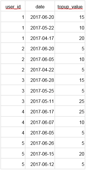
Let’s introduce some problems and demonstrate how window functions can be helpful. We will work with the following dataset: topups.tsv.
First, we create a table of top-ups. Every record represents an event of a user topping up a credit of a specified amount on a specified day.
CREATE TABLE topups (
  top_up_seq  INT PRIMARY KEY,
  user_id     INT  NOT NULL,
  date        DATE NOT NULL,
  topup_value INT  NOT NULL
);
We load the data from the file into Redshift. When using Redshift, all files have to be located in one of the Amazon storage services. The following piece of code loads a file from S3 storage using the IAM role.
COPY topups FROM 's3://<bucket-name>/<path-to-topups.tsv>'
IAM_ROLE 'arn:aws:iam::<aws-account-id>:role/<role-name>’
DELIMITER '\t';
Redshift Window Function for Month Average
We would like to compare each top-up with the average of the current month. Aggregate functions would not allow us to include topup_value in SELECT and not in GROUP BY at the same time, which is what we want. As a consequence, we would have to first compute averages over months and then join them with the original table:
WITH avg_month AS (
  SELECT
    date_part('month', date) AS month,
    date_part('year', date) AS year,
    avg(topup_value) AS average
  FROM topups
  GROUP BY date_part('month', date), date_part('year', date)
)
SELECT
  topups.user_id,
  topups.date,
  topups.topup_value,
  avg_month.average AS month_avg
FROM topups INNER JOIN avg_month
    ON avg_month.month = date_part('month', topups.date) AND
       avg_month.year = date_part('year', topups.date)
ORDER BY user_id, date DESC;
Now let’s demonstrate the solution using window functions.
SELECT user_id,
date,
topup_value,
avg(topup_value) OVER (
     PARTITION BY date_part('month', date), date_part('year', date)
     ) AS month_avg
FROM topups
ORDER BY user_id, date DESC;
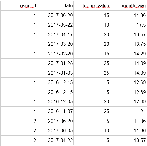
Same output for both queries. The latter approach is simpler, more elegant, and performs better.
We can check that all top-ups done in the same month have the same average. Notice that we used ORDER BY, which is completely independent of the ORDER BY that is in the OVER clause.
Redshift Window Function for Running Sum
What if we want to compute a sum of credits, that a user paid so far for each top-up? It is called a cumulative or running sum and aggregate functions are not helpful in this case. We would need the groups to be all rows with the earlier date than the current, while GROUP BY can aggregate only by the same date.
We can use sum() and customise the window to be from the first row to the current one. Dividing partitions into even smaller windows is called framing. The frames may start and end arbitrarily before or after the current row. To specify frames, the ORDER BY clause is required, so that it is determined which rows are included in each frame. Syntax for the frame definition is the following:
ROWS BETWEEN frame_start AND frame_end
where frame_start can be either UNBOUNDED PRECEDING to start from the first row or CURRENT ROW to start at the current row. Similarly frame_end can be either CURRENT ROW to end at the current row or UNBOUNDED FOLLOWING to end at the last row of the partition. Instead of ROWS we can use RANGE to define frame over values instead of rows, however, it is not fully implemented by Redshift or PostgreSQL.
When we use ordering by date, we define the frame with ROWS BETWEEN UNBOUNDED PRECEDING AND CURRENT ROW and apply sum() as window function, we get the cumulative sum over dates. Frames are being extended consecutively according to the dates. Let’s have a look at how the frames are constructed:
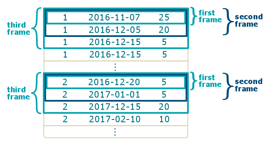
Of course, framing respects the partitions. Let’s see the solution.
SELECT user_id,
date,
topup_value,
sum(topup_value) OVER (
     PARTITION BY user_id
     ORDER BY date ROWS BETWEEN UNBOUNDED PRECEDING AND CURRENT ROW) AS total_value
FROM topups
ORDER BY user_id, date;
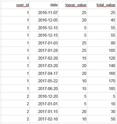
Output:
Now we can read, that e.g. the first user paid €140 by the date 2017-03-20.
Redshift row_number: Most recent Top-Ups
The task is to find the three most recent top-ups per user. To achieve it, we will use window function row_number(), which assigns a sequence number to the rows in the window. Each window, as per defined key (below user_id) is being treated separately, having its own independent sequence.
SELECT user_id, date, topup_value
FROM ( SELECT user_id,
       date,
       topup_value,
       row_number() OVER (PARTITION BY user_id ORDER BY date DESC) AS num
FROM topups) AS ranked_topups
WHERE num <= 3
ORDER BY user_id, date DESC;
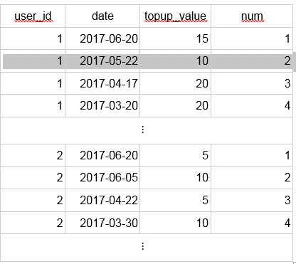
Thanks to the ORDER BY clause, the numbers are assigned consecutively according to dates. The output of the nested SELECT is the following:
Window functions operate logically after FROM, WHERE, GROUP BY, and HAVING clauses, hence we have to use outer SELECT to filter records with rank less than or equal to three.
Now let’s compute dates of the three largest top-ups ever per user. If we used row_number(), the output could miss some of the dates since users can top-up the same amount more than once. Hence, we use a window function rank(), which assigns the same rank to equal values and leaves a gap so that next values match the sequence. For a better understanding of rank(), imagine a competition in which two winners achieve the same highest score, therefore both of them are in the first place. Then the next competitor according to the score is third, not second, so the second place is unoccupied.
Redshift rank and dense_rank: Largest Top-Ups
SELECT user_id, date, topup_value, rank
FROM ( SELECT user_id,
       date,
       topup_value,
       rank() OVER (PARTITION BY user_id ORDER BY topup_value DESC) AS rank
FROM topups) AS ranked_topups
WHERE rank <= 3
ORDER BY user_id, rank;
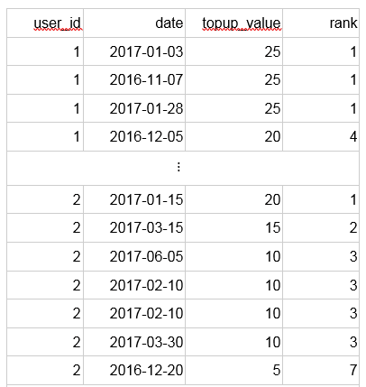
The nested SELECT produces the following output:
The rank function evaluates all of the €10 top-ups of the second user with the rank 3, as €10 is his third largest top-up.
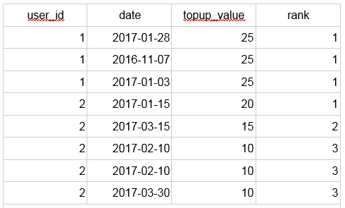
Sometimes we do not want to leave gaps in the sequence, and still assign the same rank to the equal values. Then, window function dense_rank() is what we are looking for.As we can see, all top-ups of the second user with value 10 are included. In the case of row_number(), only one of the €10 top-ups would have been included.
The following table illustrates the behaviour of all the three window functions we have mentioned:
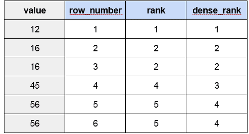
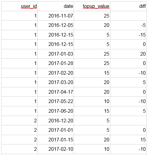
We might want to see differences of top-up values from the previous top-ups. Window function lag(expression, offset) can help us here. It accesses expression on the row prior to the current row by offset. The default offset is 1.
Redshift: Comparing row_number, rank, and dense_rankrences
SELECT user_id,
date,
topup_value,
topup_value - lag(topup_value) OVER (
     PARTITION BY user_id
     ORDER BY date, top_up_seq
) AS diff
FROM topups
ORDER BY user_id, date, top_up_seq;
Notice that we are ordering by primary key top_up_seq in the window function as well as in the final ordering – we achieve deterministic behaviour for rows with the same user and date.
Output:
The lag function is not supported by all databases. For example, Teradata database allows using only aggregate functions in the window function clause. Still, we can use aggregate function max(expression) to achieve the output with differences:The diffs at the earliest top-ups of each user are missing expectedly and the diff values correspond to the difference between current and previous row.
SELECT user_id,
date,
topup_value,
topup_value - max(topup_value) OVER (
     PARTITION BY user_id
     ORDER BY date, top_up_seq
     ROWS BETWEEN 1 PRECEDING AND 1 PRECEDING
) AS diff
FROM topups
ORDER BY user_id, date, top_up_seq;
Frame definition does not have to always contain the current row. We defined the frame as one row preceding the current. Since the frame is of size one, some other aggregate functions would work as well, e.g. min, avg, sum. The query produces the same output as the version with lag.
Uli Bethke
Uli has been rocking the data world since 2001. As the Co-founder of Sonra, the data liberation company, he’s on a mission to set data free. Uli doesn’t just talk the talk—he writes the books, leads the communities, and takes the stage as a conference speaker.
Any questions or comments for Uli? Connect with him on LinkedIn.
Follow Uli Bethke: