Improving performance and reducing costs with Materialised Views on Snowflake

Use Flexter to turn XML and JSON into Valuable Insights
- 100% Automation
- 0% Coding
What are Materialised Views?
Materialised Views are similar to Views. A View is a logical or virtual table representing the result of a query. Each time the View is queried the underlying SQL is executed and the result returned to the client. Views have the advantage of being reusable. Frequently used logic can be put into a View. Views also simplify the query logic of other SQL queries that reference the View.
Materialised Views also have these benefits. However, unlike Views they physically store the result of the underlying query in a table like structure. They precalculate the result of a query similar to ETL. Querying a Materialised View will be much faster than querying a View as the result has been precalculated and the database engine has to perform a lot less work. The downside of Materialised Views is that unlike their cousins they are not up to date and need to be refreshed whenever the data in the base tables changes.
Most databases refresh Materialised Views automatically. The database detects any changes to the underlying base tables and incrementally updates the Materialised View accordingly. Some databases only offer manual refreshes that require a full refresh of the Materialised View instead of just incrementally adding any changes.
Let’s look at the difference in performance between a View and a Materialised View.
Let’s create both of these objects
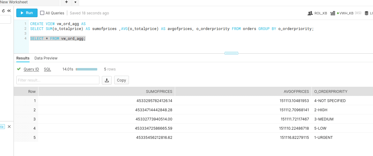
CREATE VIEW vw_ord_agg AS
SELECT SUM(o_totalprice) AS sumofprices ,AVG(o_totalprice) AS avgofprices, o_orderpriority FROM orders GROUP BY o_orderpriority;
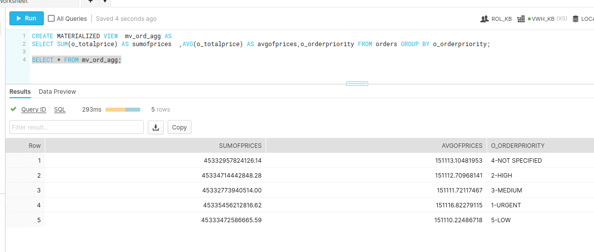
CREATE MATERIALIZED VIEW mv_ord_agg AS
SELECT SUM(o_totalprice) AS sumofprices ,AVG(o_totalprice) AS avgofprices,o_orderpriority FROM orders GROUP BY o_orderpriority;
Let’s query the View and the Materialised View and compare results
Querying the view took 14.01s
Querying materialised view took 293ms. We can see that querying MV is 47x faster
In summary
| View | Materialised View | |
|---|---|---|
| Recency | Always up to date | Needs to be refreshed |
| Results | Calculated on the fly | Physical / Materialised |
| Performance | Slower | Faster |
Oracle invented the concept of Materialised Views. They were first introduced in Oracle V8. Oracle then added the important query rewrite feature in Oracle 8i, which we will cover in a minute. Today most databases support Materialised Views.
FlowForward.
All Things Data Engineering
Straight to Your Inbox!
What are the benefits of Materialised Views?
This is all great. But how can you benefit from Materialised Views in your own queries? What are the use cases for Materialised Views? How do Materialised Views help to improve performance and save costs.
Before we dive into the use cases let’s look at one important detail I have not mentioned yet. The secret sauce of Materialised Views if you like. Databases combine Materialised Views with a feature called query rewrite. It is an awesome feature of the Cost Base Optimiser (CBO). The CBO will redirect any query against base tables to a Materialised View if it can be satisfied by the Materialised View and improves query performance. The query itself does not have to explicitly reference the Materialised View at all. It works in a similar way as an index and can significantly speed up query performance.
In the example above we created the Materialised View MV_ORD_AGG. While we can query the Materialised View directly this is pointless. We might as well have written some ETL and stored the result in any old table. Materialised Views are only useful in combination with query rewrite.
The use of Materialised Views is transparent. Users themselves don’t need to be aware of the Materialised View. The CBO will still use it if it benefits query performance.
Materialised Views by and large are only useful under the following conditions
- They are automatically refreshed in near real time
- The refresh is incremental rather than a full refresh
- The database supports the query rewrite feature
Materialised Views are similar to database indexes in that respect. Indexes also meet all of these three criteria to be useful. Just imagine you had to manually maintain an index and write queries against the index. Not very useful.
Now that we understand the benefits of Materialised Views let’s look at some general use cases. Please note that not all of these use cases are supported by all database vendors.
What are the use cases of Materialised Views?
Aggregate navigation
The original use case for Materialised Views is aggregate navigation. This was even more useful prior to columnar storage. Aggregate queries are a lot more expensive against row based storage than against columnar data storage. As a reminder, aggregate queries typically select 2-6 columns per query, which is the ideal scenario for columnar storage. Aggregate navigation is still useful today though. In particular if you are dealing with large data volumes.
Let’s have a look at what exactly we mean by aggregate navigation. A lot of the explanations and examples are taken from the excellent book Mastering Data Warehouse Aggregates. It is a bit older but still very relevant and useful today.
Aggregate tables improve query performance by reducing the number of rows the database needs to access when executing a query. Base fact tables can be summarised and store the results in a separate aggregate fact table as a Materialised View. The benefit is query performance, increased concurrency and reduced query costs. Aggregate navigation is the ability to transparently redirect queries from base tables to aggregate tables. In other words query rewrite with aggregated Materialised Views
In a star schema there are two types of aggregation. Aggregations that require an aggregate dimension and aggregations that don’t require an aggregate dimension. This is best explained by an example.
Let’s first look at an example that does not require an aggregate dimension.
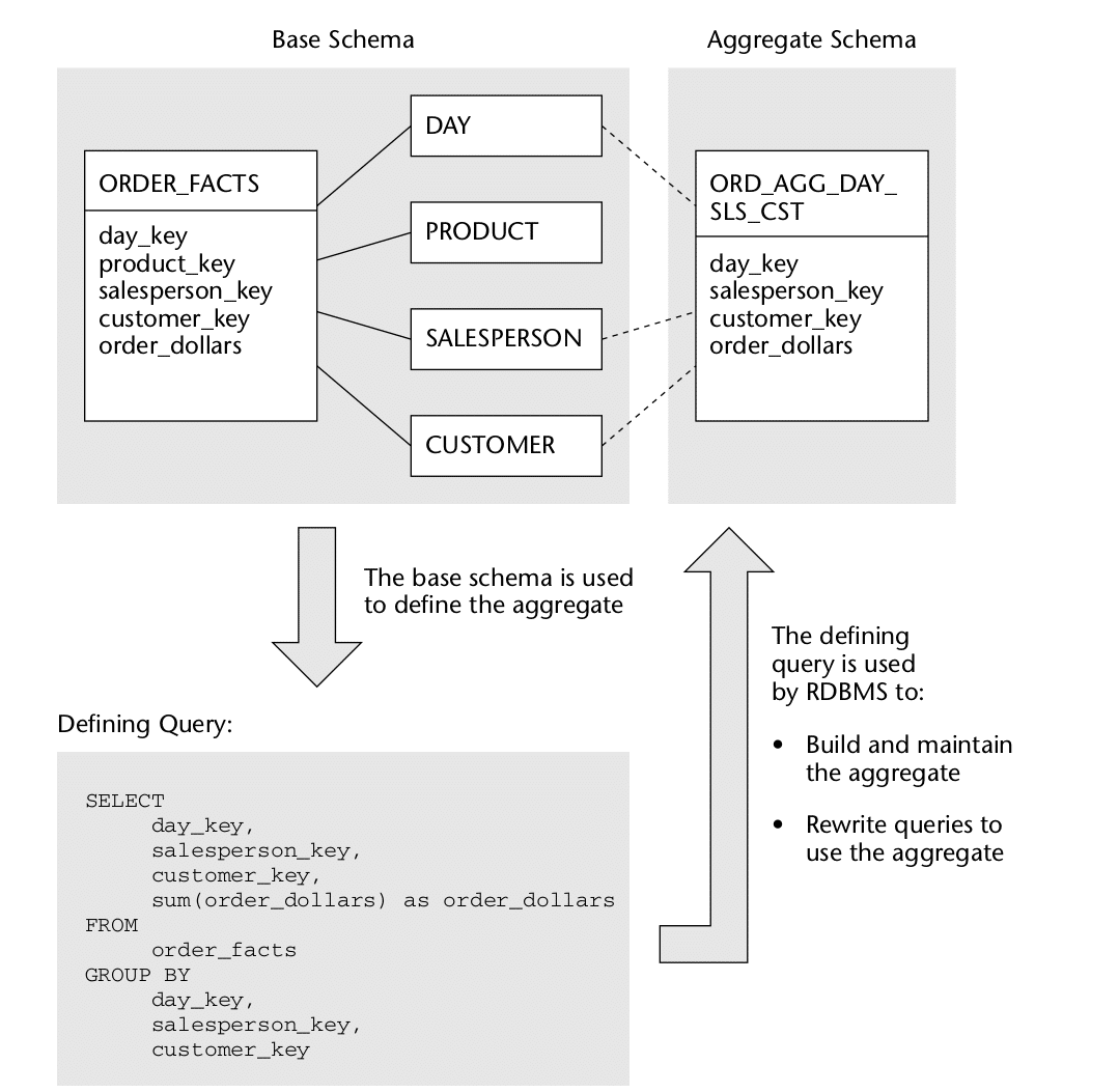
Figure taken from the excellent book Mastering Data Warehouse Aggregates.
In this example we reduce the level of granularity by removing one or more dimensions from the aggregation. In this example we aggregate by Day, Salesperson, Customer and drop the Product dimension.
Aggregate navigation with an aggregate dimension is more complex
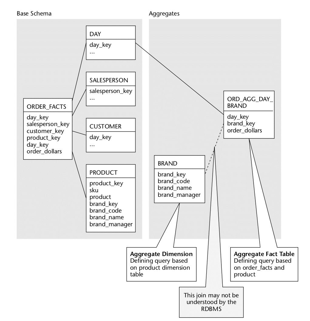
In this example (also taken from Mastering Data Warehouse Aggregates) we change the level of granularity for both the fact and the Product dimension table. For Product we aggregate on the product brand and the Order fact table we aggregate by Day and Brand. As Brand is not a dimension of the Order fact table the database CBO will not be able to rewrite our query against the aggregate table.
Some databases such as Oracle have a solution for this problem. They let you build a DIMENSION object on top of the Product dimension table that defines the rollup and drill down hierarchies (Product > Brand in this example). Using this extra bit of information the CBO can rewrite the query for scenarios with aggregate dimensions.
If your database does not support aggregate navigation for aggregate dimensions you could separate out Brand into its own conformed dimension and plug it into the Order fact table and the Order aggregate fact table.
Pre-joining data
You can pre-join data for “virtual denormalisation” or “virtual flattening” of normalised data. This is useful for scenarios where you have your data normalised but would benefit from denormalisation for performance reasons. Let me give an example where this can be useful.
You might have a large Order fact table and a large conformed Customer dimension. You can’t denormalise the Customer table into the Order table as you need the conformed Customer dimension for drill across between the Order and Order Item fact tables. By pre-joining the data you can kill two birds with one stone. You get a denormalised and prejoind Order-Customer table and you still retain the Customer dimension for drill across between the fact tables. You can expose the Customer dimension to your BI tool for query generation. The database then decides the most performant way to retrieve the data.
| Quick explainer on conformed dimensions and drill across (taken from Kimball’s book The Definitive Guide to Dimensional Modeling) |
|---|
|
Conformed dimension: Conformed dimensions are required to compare data from multiple fact tables. The set of conformed dimensions for an enterprise data warehouse is referred to as the warehouse bus. Planned in advance, the warehouse bus avoids incompatibilities between subject areas. 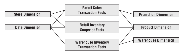
Drill across: In addition to consistency and reusability, conformed dimensions enable you to combine performance measurements from different business processes in a single report. You can use multipass SQL to query each dimensional model separately and then outer-join the query results based on a common dimension attribute such as product name. The full outer-join ensures all rows are included in the combined report, even if they only appear in one set of query results. This linkage, often referred to as drill across, is straightforward if the dimension table attribute values are identical. 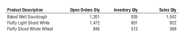
Drill across three fact tables using the Product dimension |
Pre-joining data only works with INNER JOINs. It is one of the many limitations of Materialised Views that we will explore further down.
Lookups and range queries
Relational databases for OLTP have B-tree indexes for looking up individual values and for range queries. Columnar databases for data analytics typically don’t support B-tree indexes.
The primary use case for data analytics and data warehousing is to scan large volumes of data for reporting purposes. However, lookups, filtering and range queries are still common scenarios.
For lookups, columnar databases provide storage indexes. One implementation of a storage index are the stats kept at the micro partition level on Snowflake. While these help and work particularly well for unique values, they are not as efficient as a Btree index. We also have cluster or sort keys. Cluster keys presort the data and as a result increase the efficiency of storage indexes. However, you can only have one cluster key per table (albeit with multiple columns).
For scenarios where you can benefit from multiple cluster keys for lookups and range queries of columns with medium-high to high cardinality (lots of distinct values) you can create Materialised Views with additional cluster keys.
As far as I know this concept of multiple sort keys was first introduced by Vertica and can now be found in many other databases such as Snowflake etc.
Hot and cold data. Data archive
You may have tables with hot and cold data, i.e. a smaller subset of the data is queried frequently while some older data is rarely or never queried. Think of a data archive. Rather than splitting the data across a current and an archive table you want to keep the data in the same table to make it easier for data consumers to query the data.
If your database supports table partitions then Materialised Views are not a good fit and you are better off using table partitions. However, if your database does not support table partitions then a Materialised View over the current data is a good fit for this use case.
| Base table | Materialised View |
|---|---|
| Hot / current data | Hot / current data |
| Cold / archive data |
Any queries against the base table that filter on the column that filters against value current=true will be redirected to the Materialised View and has to scan significantly less data, which in turn will speed up the queries.
Semi-structured data
Support for querying JSON was introduced a couple of years ago to the SQL ANSI standard. Most relational databases now have support for querying and parsing JSON.
Parsing JSON on the fly can be slow and you can speed up the process with Materialised Views.
External tables
In many cases, Materialised Views over external tables provide better performance than direct queries over the underlying external table. This performance difference can be significant when a query is run frequently or is complex.
You will need to check if your database supports Materialised Views over external tables. The other important item to check is that the underlying data for the external table can be automatically refreshed, e.g. this is possible in Snowflake.
Stateful streaming
Another interesting use case for Materialised Views is stateful streaming. You can build a Materialised View on top of a stream of real time data and automatically and incrementally “refresh” your stateful calculations, e.g. you can calculate the total number of daily visitors on top of a clickstream using a Materialised View. This works well for additive metrics.
COUNT DISTINCT queries
COUNT DISTINCT is a computationally expensive operation and decreases database performance. That is the reason why BigQuery defaults to an approximate distinct count (HyperLogLog) when the user issues a DISTINCT COUNT clause in a SQL statement. BigQuery provides a function exact_count_distinct for exact distinct count results. However, this is not the default version!
One of two algorithms is typically used for distinct counts.
- Sorting: Records are sorted, duplicate records then are identified and then removed. The number of target expression values in the remaining set of tuples would then represent a distinct count of the target expression values.
- Hashing: Records are hashed and then duplicates are removed within each hash partition. Implementing hashing may be less computationally intensive than the sorting approach and may scale better with a sufficiently large set of records. However, it is still computationally expensive
Another approach is bitmap-based count distinct in SQL. It can be calculated at runtime. However, you get the most benefits when you combine it with a Materialised View. You can then precompute and incrementally refresh the results.
Bitmap based count distinct It can be used in combination with a Materialised View (incrementally refreshed).
Limitations of Materialised Views
Materialised Views that refresh incrementally have limitations. These limitations are not vendor specific but are a shared characteristic of incremental Materialised Views.
Let’s have a look at some common limitations:
- No support for outer joins. Some databases don’t support any joins including inner joins.
- No support for window functions
- No support for the DISTINCT clause
- No support for non-additive aggregate functions, e.g. MEDIAN. Additive aggregate functions such as SUM, AVG etc are supported.
- No support for nesting of aggregate functions
You can probably see a common pattern here. Materialised Views do not support any features that require the database to recalculate parts of the Materialised View during the incremental refresh operation. Any operation or calculation that needs to look across the delta of new data versus existing data in the Materialised View is not supported.
The supported features are typically good for simpler operations and transformations. More complex calculations which are the majority of transformations in a data warehouse are not supported. As we have seen, Materialised Views are still useful for many scenarios and use cases.
Incrementally refreshing a Materialised View shares some of the same limitations as stateful real time analytics. Anything other than non-trivial transformations are difficult or impossible as they require work on all of the data and not just incremental data. Let’s go through an example.
In this table we have a list of customer orders.
| customer_id | order_amount |
|---|---|
| 1 | 10 |
| 1 | 25 |
| 1 | 50 |
| 2 | 45 |
| 3 | 21 |
| 3 | 56 |
Number of orders: 6
Number of distinct customers with orders: 3
A couple of new orders arrive
| customer_id | order_amount |
|---|---|
| 5 | 10 |
| 1 | 67 |
Calculating the total number of orders is easy. We just count the number of new orders and add them to the number of existing orders. There is no need to look at each single record across the whole window.
Number of orders = Number of existing orders + number of new orders
6 + 2 = 8
Calculating the number of distinct customers is more tricky. We need to look at the existing orders and can not just add the number of distinct customers from the new orders. In other words the number of distinct customers is not additive.
Translated to the world of the Materialised View we can not incrementally refresh the Materialised View for distinct counts. We would need to fully refresh the resultset. As this is an expensive operation it is not supported for incremental refreshes.
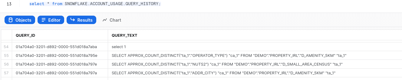
How to detect candidates for Materialised Views?
When looking for candidate queries for Materialised Views you need to analyse the SQL queries that your users run inside the database.
Most relational databases have an information schema where they log the history of any SQL statements that users run and tools generate.
On Snowflake the history of SQL statements is stored in the query_history table in the account_usage schema.
Zoom in on the following criteria for finding candidates:
- Focus on queries that are slow in comparison to other queries
- Look for queries that
- Identify the WHERE, GROUP BY and JOIN clause columns. Aggregate the information and check for those columns that repeatedly and frequently show up. These are your candidates.
Once you have identified candidates run some tests by creating Materialised Views. Check the performance improvement on aggregate across all of the queries that can be rewritten by the CBO against the Materialised Views.
You can use the online SQL parser component of our SQL data processing tool FlowHigh to easily identify candidates for Materialised Views.
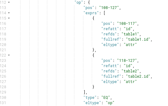
Let’s take the following query as an example and parse it with FlowHigh
SELECT table1.col1
,table2.col2
,SUM(table2.col3) sum_col3
FROM table1
JOIN table2
ON(table1.id=table2.id)
WHERE table2.col4=12
GROUP BY table1.col1
,table2.col2;
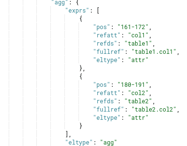
… and here is the output of the SQL parser
Join columns
Filter column
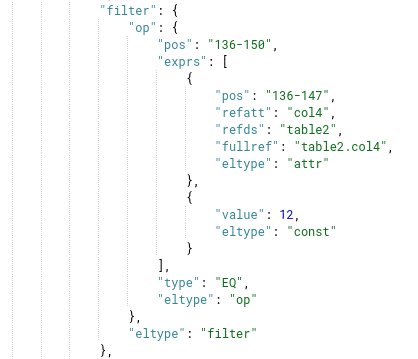
Aggregate columns
Materialised Views on Snowflake
Snowflake has an advanced Cost Based Optimiser (CBO). It can rewrite a query against a base table and redirect it to a Materialised View to improve performance.
Let’s look at a couple of use cases of Materialised Views on Snowflake
For all of the use cases we used tables from the Snowflake sample_data database in schema TPCH_SF1000. You can sign up for a free trial of Snowflake and try out the examples yourself.
Use case 1: Data archive. Hot versus cold data
Data archive is a good use case for Snowflake as it does not have a table partition feature.
In this example, we will use the ORDERS table with 1.5 billion rows. It is about 38.9 GB in size (compressed).
For testing purposes, we switch off result caching.
ALTER SESSION SET USE_CACHED_RESULT=FALSE;
For this business scenario 95% of the queries that are executed against the ORDERS table filter for urgent orders. Urgent orders are hot. Any other orders are cold and have been archived and are queried infrequently. This is a good scenario for a Materialised View.
Let’s assume we want to see the number of orders handled by each clerk in the urgent orders.
We can query it from the base table as follows:
SELECT o_clerk, COUNT(*) FROM order_original WHERE o_orderpriority = '1-URGENT' group by o_clerk;
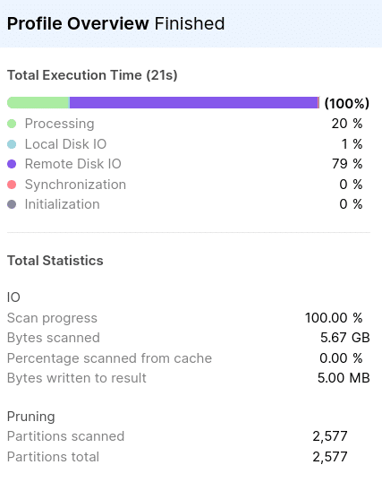
It took snowflake 21,77 s to run this query. Looking under the hood using EXPLAIN we can see that the query requires a full table scan.
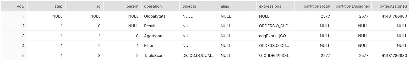
2,577 of 2,577 micro partitions were scanned.
Now let’s create a Materialised View with all the urgent orders as MV_URGENT_ORDERS.
CREATE MATERIALIZED VIEW mv_urgent_orders AS
SELECT * FROM orders WHERE o_orderpriority = '1-URGENT';
MV_URGENT_ORDERS now holds the result set of all urgent orders. After creating the MV, we run the previous SELECT query against the base table to check performance.
SELECT o_clerk, COUNT(*) FROM order_original WHERE o_orderpriority = '1-URGENT' group by o_clerk;
It took just 10.7s to run the query. This is about twice as fast as the previous query. What happened?
Let’s check the EXPLAIN command.
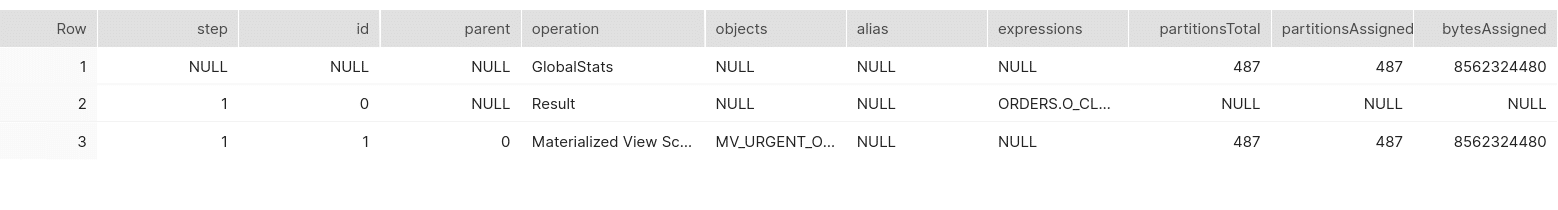
We can see that even though we didn’t specify the Materialised View in the SQL statement the query optimiser automatically rewrote the query. It redirected it from the base table to the MV. This dramatically speeds up query performance.
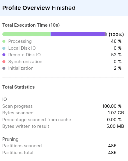
The following screenshot was taken from the QUERY_PROFILE and shows that the query improved drastically after creating the MV_URGENT_ORDERS. Compared to the previous execution, the total number of Partitions and Bytes scanned is reduced five times.
Search optimisation and cluster keys as alternatives to Materialised Views for archived data?
Instead of creating a Materialised View to speed up performance we can use cluster keys or search optimisation for data archive scenarios. However, for binary search scenarios (urgent vs. non-urgent or archive vs. non-archive or cold vs hot data) cluster keys or search optimization are not a good fit. The cardinality (number of distinct values) is likely too low. Cluster keys require sorting and are more expensive to create and refresh for this scenario than Materialised Views.
Use case 2: Materialised Views for lookups and filters
With a Materialised View we can create alternative cluster keys on a single table. You can have a cluster key on your primary table and then one or more additional cluster keys by creating a Materialised View. The usual considerations for creating cluster keys apply.
A cluster key sorts a table by the cluster columns and reduces the number of micro partitions that need to be scanned when filtering data. You can only have one cluster key per table. However, you can define additional cluster keys on a table through a Materialised View.
You can cluster the Materialised View on different columns than the columns used to cluster the base table. This helps us define multiple cluster keys for the same table and hence improves the performance when filtering or joining data.
Let’s dive into this with an example.
We use the ORDERS table from the previous example to create sample datasets for this test case.
We create a table clustered by the O_CLERK column
CREATE TABLE clustered_orders LIKE orders;
ALTER TABLE clustered_orders CLUSTER BY (o_clerk);
INSERT INTO clustered_orders SELECT * FROM orders;
Now, let’s derive a Materialised View from this table with a cluster key on a different column.We will take ORDER_DATE_NUM as the candidate for this key.
CREATE MATERIALIZED VIEW mv_clustered_orders CLUSTER BY (order_date_num) AS SELECT * FROM clustered_orders ;
Let’s now check a scenario where we want to look up some data based on the filter condition ORDER_DATE_NUM.
The optimiser knows that the base table is clustered by O_CLERK whereas the derived MV by ORDER_DATE_NUM. For best performance the CBO redirects the query against the base table to the MV for better performance.
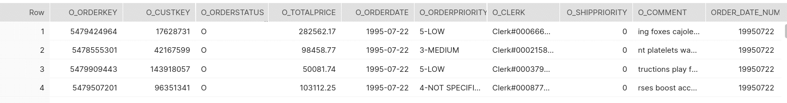
EXPLAIN SELECT * FROM clustered_orders WHERE order_date_num =19950722;
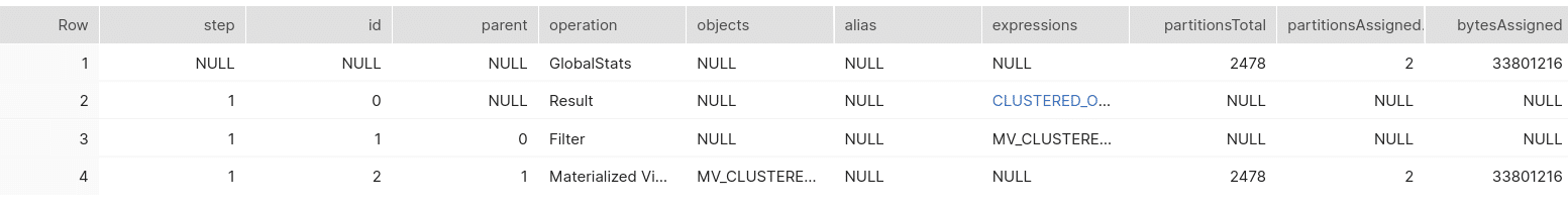
As the execution plan suggests even though we queried against the base table the query was redirected to the MV.
Search optimisation as an alternative to Materialised Views for lookups?
Instead of creating a Materialised View to speed up performance we can use search optimisation for lookup operations. When deciding between search optimisation and cluster keys consult the Snowflake documentation. As a general rule storage indexes (micro partitions) work best for very high cardinality columns (unique keys work best). Search optimisation works best for high cardinality columns and cluster keys best for medium-high to high cardinality columns. You can combine cluster keys with Materialised Views to get around the limitation of one cluster key per table.
high cardinality means that there are a lot of distinct values in the column.
You can also consult the following links when deciding between cluster keys and search optimisation.
Use case 3: Aggregate Navigation with MVs
In data warehouses, materialised views normally contain aggregates. Let’s see how Snowflake handles aggregate navigation with Materialised Views.
Let’s take another sample scenario from the Orders table.
Let’s consider the following aggregate query with a SUM and AVG.
SELECT SUM(o_totalprice) AS sumofprices, AVG(o_totalprice) AS avgofprices, o_orderpriority FROM orders GROUP BY o_orderpriority;
It took Snowflake 15 seconds to run this query.
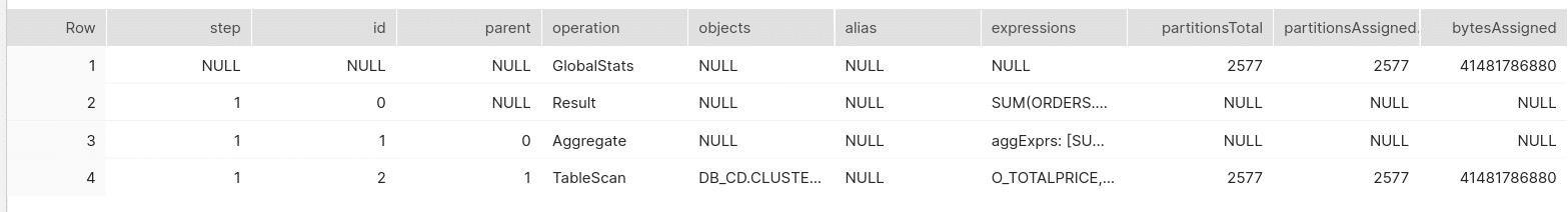
Investigating the execution plan we see that all table partitions were scanned.
Let’s create a Materialised View that pre-aggregates data
CREATE MATERIALIZED VIEW mv_agg AS
SELECT SUM(o_totalprice) AS sumofprices ,AVG(o_totalprice) AS avgofprices, o_orderpriority FROM orders GROUP BY o_orderpriority;
Now let’s test the same query performance after the creation of this MV.
SELECT SUM(o_totalprice) AS sumofprices , AVG(o_totalprice) AS avgofprices, o_orderpriority FROM orders GROUP BY o_orderpriority;
It just took 678 ms to produce this result. As you’ve guessed the query is redirected to the MV where we have already pre aggregated the data.
Let’s confirm it by viewing the explain plan.
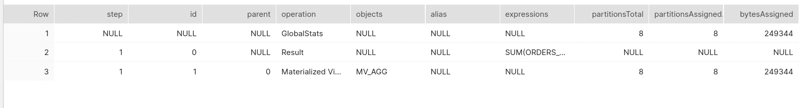
Well, that’s not all. The query optimiser can also use the Materialised View for queries at a higher level of granularity and queries with filters against o_orderpriority.
Say we need the total price for medium priority orders :
SELECT SUM(o_totalprice) FROM orders WHERE o_orderpriority ='3-MEDIUM';
We don’t even have to GROUP BY o_orderpriority as the query is at a higher level of granularity than the Materialised View. Snowflake still redirects the query.
The difference in execution time before and after creating MV for this query changes from 13.46s to 338ms. The creation of MV accelerates the query by ~20x.
Use case 4: pre-joining data
Snowflake does not support inner joins when creating a Materialised View. Unfortunately, we can’t use Materialised Views for pre-joining data and pre-calculating expensive inner joins at the moment.
Use case 5: bitmap based count distinct
You can use a Materialised View in combination with bitmap based count distinct to speed up count distinct queries. The Snowflake documentation discusses bitmap based count distinct in detail. In summary you can use bitmaps and bitmap buckets to keep track of distinct values in a table. You can then use bitmap aggregate functions to summarise the distinct values.
Let’s go through an example. We are using the sample data TPCH provided by Snowflake
CREATE OR replace MATERIALISED VIEW mv_partkey_cntdist AS
SELECT
l_partkey,
BITMAP_BUCKER_NUMBER(l_quantity) bucket,
BITMAP_CONSTRUCT_AGG(bitmap_bit_position(l_quantity)) bmp
FROM lineitem
GROUP BY l_partkey, bucket;
Query formatted with FlowHigh formatter
We created a bitmap and bitmap bucket for the l_quantity column grouped by l_partkey
Let’s have a look at the data inside the Materialised View
Select * FROM mv_partkey_cntdist;
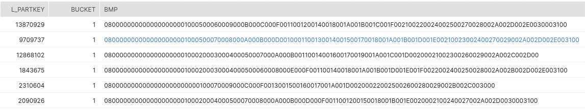
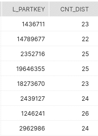
It contains a bucket and bitmap which we can use with bitmap aggregate functions to determine the distinct count for l_quantity grouped by l_partkey.
SELECT l_partkey
,SUM(cnt) cnt_dist
FROM( SELECT l_partkey
,BITMAP_COUNT(BITMAP_CONSTRUCT_AGG(BITMAP_BIT_POSITION(l_quantity))) cnt
FROM lineitem
GROUP BY l_partkey
,BITMAP_BUCKET_NUMBER(l_quantity))
GROUP BY l_partkey;
Unfortunately, the Snowflake CBO does not rewrite count distinct queries against the Materialised View and currently you need to query the Materialised View directly.
The following query will not get redirected to the Materialised View
SELECT l_partkey, COUNT(DISTINCT l_quantity) FROM lineitem GROUP BY l_partkey;
Parsing semi-structured data
You can create a Materialised View on top of complex JSON to increase query performance against JSON data. However, we recommend converting any frequently queried JSON or XML data to a relational format instead. We have created a Flexter to automate the conversion of XML and JSON to a readable format on Snowflake in seconds. Any type. Any volume.
External tables – Data Lake speed up
If you have built a data lake on object storage and created Snowflake external tables on top of it you can use Materialised VIews to speed up access to those tables
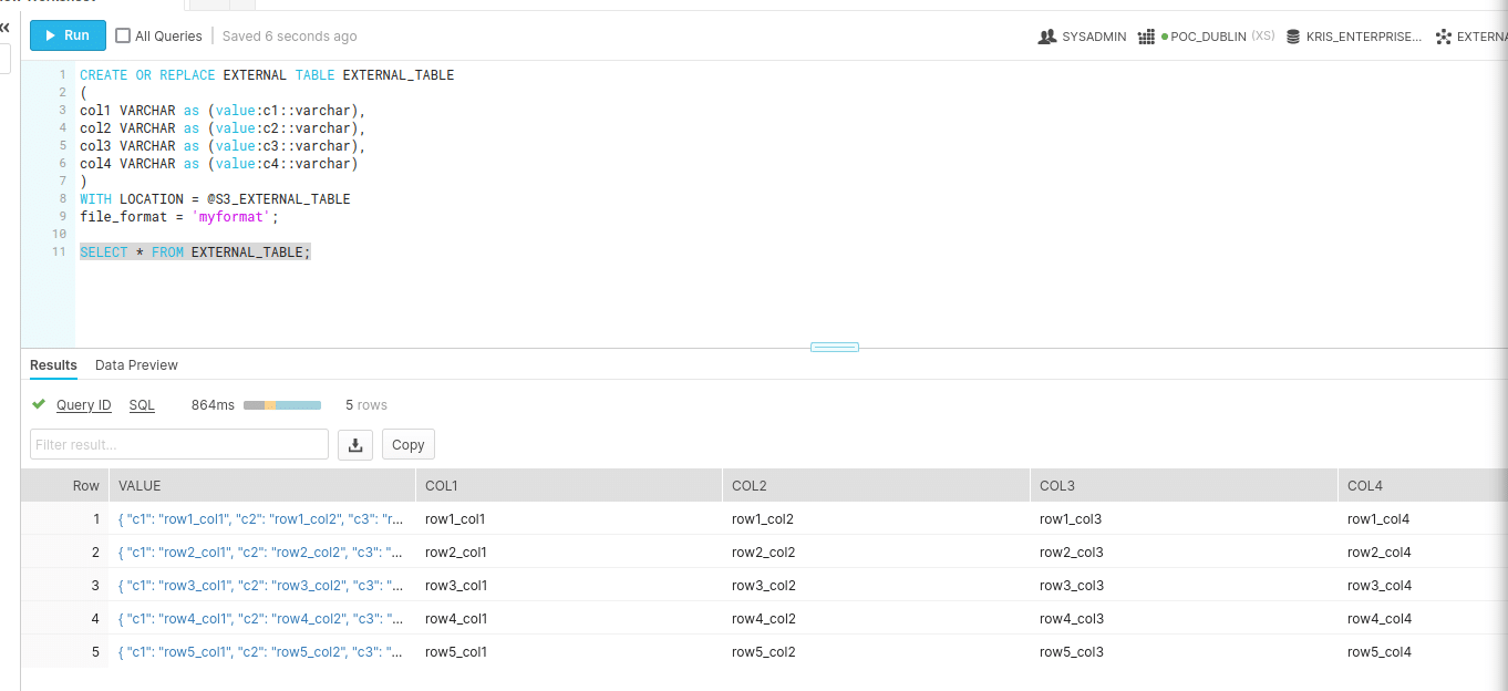
First create an external table from a Stage S3_EXTERNAL_TABLE.
CREATE OR REPLACE EXTERNAL TABLE external_table
(
col1 VARCHAR as (value:c1::varchar),
col2 VARCHAR as (value:c2::varchar),
col3 VARCHAR as (value:c3::varchar),
col4 VARCHAR as (value:c4::varchar)
)

WITH LOCATION = @S3_EXTERNAL_TABLE
file_format = 'myformat';

SELECT * FROM external_table;
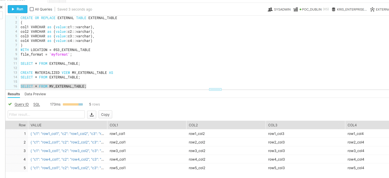
Next we creating the Materialised View (MV_EXTERNAL_TABLE)
CREATE OR REPLACE EXTERNAL TABLE external_table
(
col1 VARCHAR as (value:c1::varchar),
col2 VARCHAR as (value:c2::varchar),
col3 VARCHAR as (value:c3::varchar),
col4 VARCHAR as (value:c4::varchar)
)

WITH LOCATION = @S3_EXTERNAL_TABLE
file_format = 'myformat';

SELECT * FROM external_table;

CREATE MATERIALIZED VIEW mv_external_table AS
SELECT * FROM external_table;

SELECT * FROM mv_external_table;
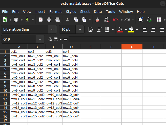
Next we add some more data to the external table in the form of a CSV file
We check that the data is refreshed in the external table.
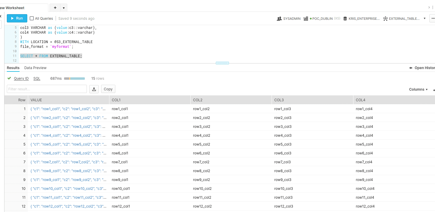
The query shows the newly added rows
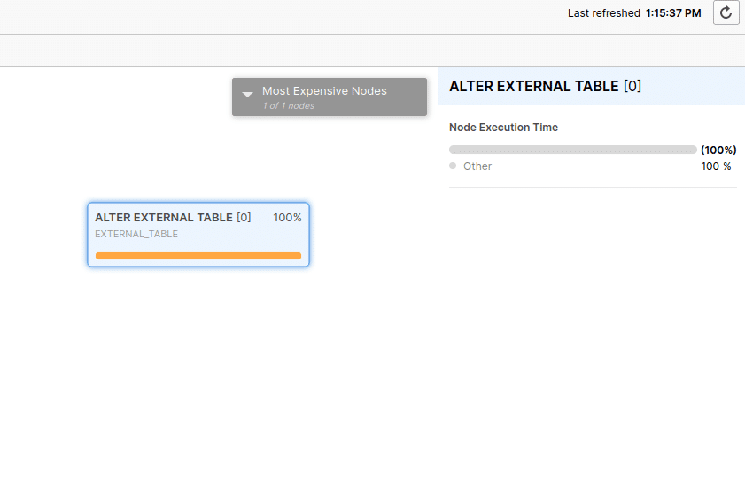
Next we check that the Materialised View (MV_EXTERNAL_TABLE) was refreshed
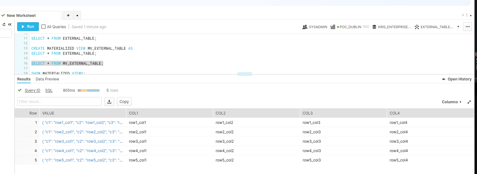
The MV still shows the old results
Run refresh on EXTERNAL_TABLE
ALTER EXTERNAL TABLE external_table REFRESH;
Select all data from Materialised view MV_EXTERNAL_TABLE
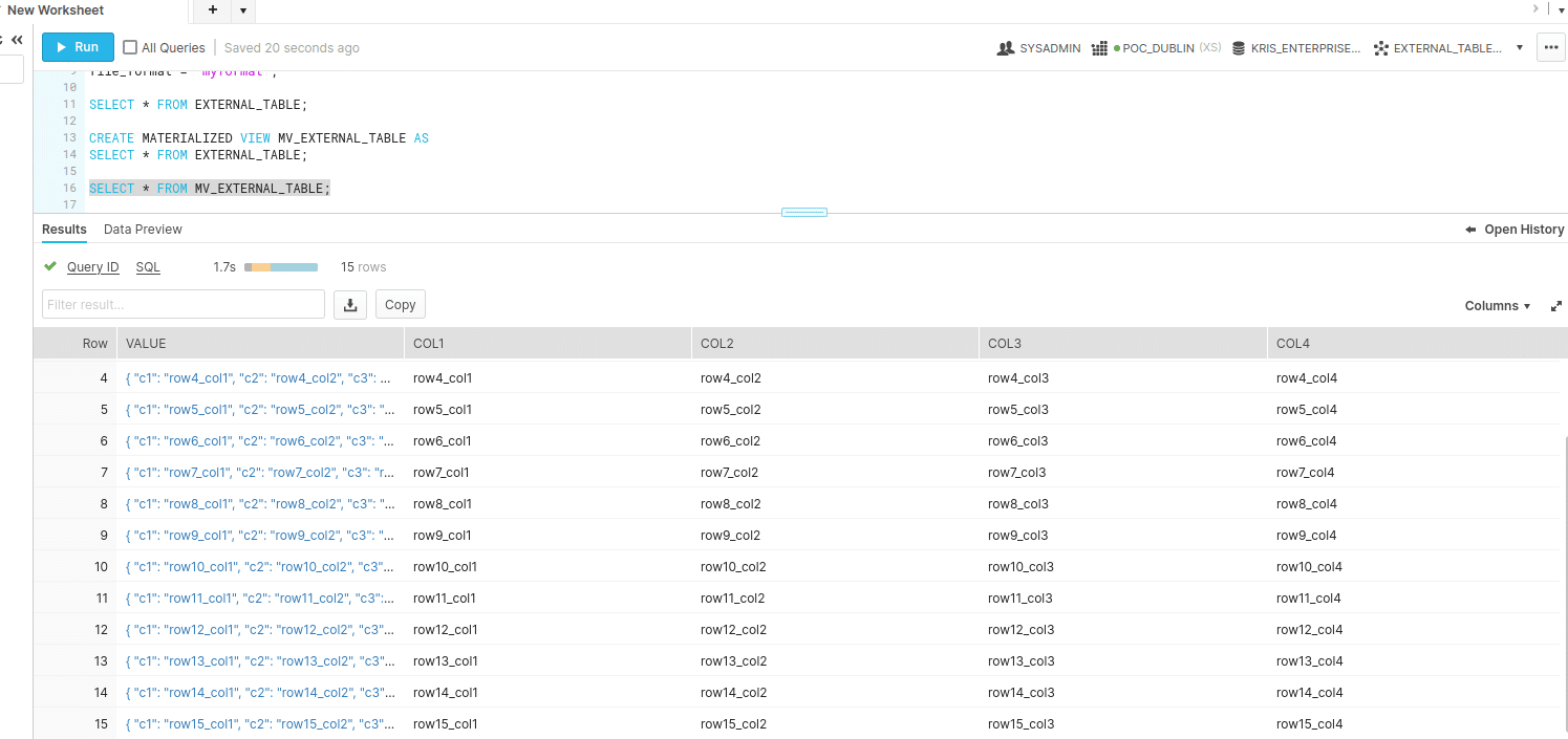
The Materialised View was refreshed
Get practical about Materialised Views
Now you know everything you ever need to know about Materialised Views. Why not put all your new knowledge into practice and start saving money with Materialised Views.
Use FlowHigh to identify SQL candidate queries for Materialised Views. Use it to optimise, visualise, format, parse SQL queries. And for data lineage.
can you add this at the end of the post
Uli Bethke
Uli has been rocking the data world since 2001. As the Co-founder of Sonra, the data liberation company, he’s on a mission to set data free. Uli doesn’t just talk the talk—he writes the books, leads the communities, and takes the stage as a conference speaker.
Any questions or comments for Uli? Connect with him on LinkedIn.
Follow Uli Bethke: