Deep dive on SQL parsing on Teradata

October 19, 2023

This is the sixth article in our series on parsing SQL in different database technologies and SQL dialects. We explored SQL parsing on Snowflake, MS SQL Server, Oracle , Databricks ,Redshift and AWS Athena in our earlier blog posts. We cover SQL parsing in Teradata in this blog post and go through a practical example of table and column audit logging.

Table of Contents

We provide practical examples of deconstructing SQL from the Teradata history. Additionally, we will present some code that utilises the FlowHigh SQL parser SDK to programmatically parse SQL from Teradata. The parsing of sql from Teradata can be automated using the SDK.

In another post on the Sonra blog, I go into great depth on the use cases of using an SQL parser for data engineering and data governance use cases. The mentioned article is a complete deep dive into SQL parsing, how it works and how you can use it for use cases in data engineering and data governance.

SQL parser for Teradata

Sonra has created an online SQL parser. Our vision is to be SQL dialect agnostic. The parser also works with Teradata. It is called FlowHigh. Our SaaS platform includes a UI for manual SQL parsing as well as an SDK for managing bulk SQL parsing requirements or automating the process. We demonstrate FlowHigh’s capabilities by parsing the query history of Teradata.

Let’s look at both options starting with the SDK for automating SQL parsing.

Programmatically parsing the Teradata query history with the FlowHigh SDK

We used a Teradata Vantage cloud hosted instance. This resource enables us to explore, test, and develop without a local Teradata setup. Teradata Vantage is available at https://clearscape.teradata.com. You can check out Teradata’s capabilities, play with queries, and build prototypes in an environment that mirrors a full-scale Teradata deployment. It offers a practical and convenient way for developers and analysts to hone their skills and run test cases in a real-world Teradata environment.

We used this environment to iterate over the Teradata query history and parse the submitted SQL. The query history is contained in QryLogSQLV.

QryLogSQLV is a system view residing within the DBC database to store and present detailed information about the SQL queries executed in the Teradata environment. Specifically, QryLogSQLV focuses on capturing and displaying the SQL text of queries.

We can query QryLogSQLV to retrieve information about the executed SQL queries on Teradata database using the below query.

SELECT
	QueryID, SqlTextInfo
FROM
	DBC.QryLogSQLV
ORDER BY
	CollectTimeStamp

SELECT

QueryID, SqlTextInfo

FROM

DBC.QryLogSQLV

ORDER BY

CollectTimeStamp

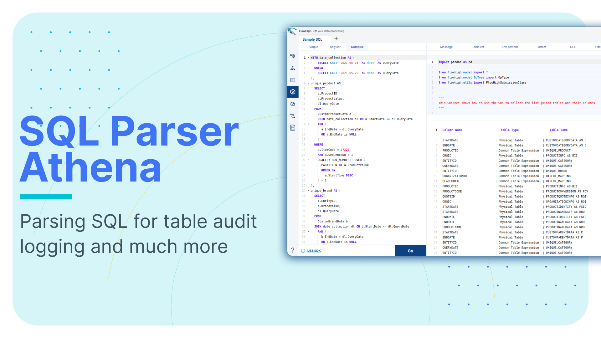
The python code in the next section shows how the query history is pulled from AWS Athena and processed using the FlowHigh SDK:

import teradatasql
import pandas as pd
from flowhigh.utils.converter import FlowHighSubmissionClass
# Connection parameters
host = 'hostname'
user = 'username'
password = 'password'

# Connection string
con_str = f'{{"host":"{host}","user":"{user}","password":"{password}"}}'

# SQL query to retrieve query logs
query = """
SELECT QueryID, SqlTextInfo from DBC.QryLogSQL
"""

# Create a connection
con = teradatasql.connect(con_str)

# Create a cursor from the connection
cur = con.cursor()
cur.execute(query)
row = cur.fetchall()
print(row)
data =[]
for i in row:
	fh = FlowHighSubmissionClass.from_sql(i[1])
	json_msg = fh.json_message
	entry = {'query_id': i[0], 'fh_response': json_msg}
	data.append(entry)
	print(data)

data_df = pd.DataFrame(data)
print(data_df)

cur.close()
con.close()

import teradatasql

import pandas as pd

from flowhigh.utils.converter import FlowHighSubmissionClass

# Connection parameters

host = 'hostname'

user = 'username'

password = 'password'

# Connection string

con_str = f'{{"host":"{host}","user":"{user}","password":"{password}"}}'

# SQL query to retrieve query logs

query = """

SELECT QueryID, SqlTextInfo from DBC.QryLogSQL

"""

# Create a connection

con = teradatasql.connect(con_str)

# Create a cursor from the connection

cur = con.cursor()

cur.execute(query)

row = cur.fetchall()

print(row)

data =[]

for i in row:

fh = FlowHighSubmissionClass.from_sql(i[1])

json_msg = fh.json_message

entry = {'query_id': i[0], 'fh_response': json_msg}

data.append(entry)

print(data)

data_df = pd.DataFrame(data)

print(data_df)

cur.close()

con.close()

Analysing the output of the FlowHigh SQL parser

The FlowHigh SQL parser for Teradata analyses the SQL queries you submit and delivers the output as a JSON or XML message. The output message contains information about filter parameters, fetched columns, aliases, join conditions, tables, and any other SQL command clauses used in the query.

Let’s go through an example. We will use a simple SQL query to demonstrate some of the features of the parser.

SELECT C.CustomerName
     ,O.OrderDate
     ,COUNT(DISTINCT O.OrderId) AS NumberOfOrders
     ,SUM(OD.Quantity) AS TotalQuantityOrdered
 FROM Customers C
 JOIN Orders O
   ON C.CustomerId=O.CustomerId
 JOIN OrderDetails OD
   ON O.OrderId=OD.OrderId
WHERE O.OrderDate>='2023-01-01'
  AND O.OrderDate<='2023-12-31'
GROUP BY C.CustomerName
     ,O.OrderDate
HAVING SUM(OD.Quantity)>10
ORDER BY TotalQuantityOrdered DESC;

SELECT C.CustomerName

,O.OrderDate

,COUNT(DISTINCT O.OrderId) AS NumberOfOrders

,SUM(OD.Quantity) AS TotalQuantityOrdered

FROM Customers C

JOIN Orders O

ON C.CustomerId=O.CustomerId

JOIN OrderDetails OD

ON O.OrderId=OD.OrderId

WHERE O.OrderDate>='2023-01-01'

AND O.OrderDate<='2023-12-31'

GROUP BY C.CustomerName

,O.OrderDate

HAVING SUM(OD.Quantity)>10

ORDER BY TotalQuantityOrdered DESC;

The SQL parser also supports other DML and DDL statements such as CREATE, INSERT, UPDATE, MERGE etc.

Let’s examine the XML output from the FlowHigh SQL parser for the given SQL query. This XML format is more concise than its JSON cousin. Both types of messages have the same content though.

<?xml version="1.0" encoding="UTF-8"?>
<parSeQL version="1.0" status="OK" ts="2023-10-05T11:02:51.310Z" xmlns:xsi="http://www.w3.org/2001/XMLSchema-instance" xsi:schemaLocation="https://flowhigh.sonra.io/flowhigh_v1.0.xsd">
  <statements>
	<statement pos="0-449">
  	<ds pos="0-449" type="root" subType="inline">
    	<out>
      	<attr pos="12-14" oref="C1"/>
      	<attr pos="32-11" oref="C2"/>
      	<func xsi:type="fagg" pos="49-43" alias="NumberOfOrders" name="COUNT" quantifier="DISTINCT">
        	<attr pos="64-9" oref="C3"/>
      	</func>
      	<func xsi:type="fagg" pos="98-40" alias="TotalQuantityOrdered" name="SUM">
        	<attr pos="102-11" oref="C4"/>
      	</func>
    	</out>
    	<in>
      	<ds pos="149-11" alias="C" oref="T1"/>
      	<join type="inner" definedAs="explicit">
        	<ds pos="171-8" alias="O" oref="T2"/>
        	<op pos="183-27" type="EQ">
          	<attr pos="183-12" oref="C5"/>
          	<attr pos="198-12" oref="C6"/>
        	</op>
      	</join>
      	<join type="inner" definedAs="explicit">
        	<ds pos="221-15" alias="OD" oref="T3"/>
        	<op pos="240-22" type="EQ">
          	<attr pos="240-9" oref="C3"/>
          	<attr pos="252-10" oref="C7"/>
        	</op>
      	</join>
    	</in>
    	<filter xsi:type="filtreg">
      	<op pos="274-59" type="AND">
        	<op pos="274-27" type="GTE">
          	<attr pos="274-11" oref="C2"/>
          	<const>'2023-01-01'</const>
        	</op>
        	<op pos="306-27" type="LTE">
          	<attr pos="306-11" oref="C2"/>
          	<const>'2023-12-31'</const>
        	</op>
      	</op>
    	</filter>
    	<agg xsi:type="aggreg">
      	<attr pos="348-14" oref="C1"/>
      	<attr pos="364-11" oref="C2"/>
    	</agg>
    	<filter xsi:type="filtagg">
      	<op pos="388-21" type="GT">
        	<func xsi:type="fagg" pos="388-16" name="SUM">
          	<attr pos="392-11" oref="C4"/>
        	</func>
        	<const>10</const>
      	</op>
    	</filter>
    	<sort>
      	<attr pos="424-20" direction="desc" sref="98-40" oref="C4"/>
    	</sort>
  	</ds>
  	<antiPatterns type="AP_02">
    	<pos>49-43</pos>
  	</antiPatterns>
	</statement>
  </statements>
  <DBOHier>
	<dbo oid="T1" type="TABLE" name="Customers">
  	<dbo oid="C1" type="COLUMN" name="CustomerName"/>
  	<dbo oid="C5" type="COLUMN" name="CustomerId"/>
	</dbo>
	<dbo oid="T2" type="TABLE" name="Orders">
  	<dbo oid="C2" type="COLUMN" name="OrderDate"/>
  	<dbo oid="C3" type="COLUMN" name="OrderId"/>
  	<dbo oid="C6" type="COLUMN" name="CustomerId"/>
	</dbo>
	<dbo oid="T3" type="TABLE" name="OrderDetails">
  	<dbo oid="C4" type="COLUMN" name="Quantity"/>
  	<dbo oid="C7" type="COLUMN" name="OrderId"/>
	</dbo>
  </DBOHier>
</parSeQL>

<?xml version="1.0" encoding="UTF-8"?>

<out>

</func>

</func>

</out>

<in>

</op>

</join>

</op>

</join>

</in>

</op>

</op>

</filter>

</agg>

</func>

</op>

</filter>

<sort>

</sort>

</ds>

</antiPatterns>

</statement>

</statements>

</dbo>

</dbo>

</dbo>

</DBOHier>

</parSeQL>

The XML output generated by the FlowHigh SQL parser for AWS Athena provides an in-depth analysis of the SQL statement.

Tables and columns

The XML outlines references to three tables used in the query: Customers, Orders, and OrderDetails, each of which is shown with a unique identifier in the DBOHier section of the XML message. The columns involved from these tables are as follows:

From the Customers table: CustomerName and CustomerId.
From the Orders table: OrderDate and OrderId.
From the OrderDetails table: Quantity and OrderId.

 <DBOHier>
	<dbo oid="T1" type="TABLE" name="Customers">
  	<dbo oid="C1" type="COLUMN" name="CustomerName"/>
  	<dbo oid="C5" type="COLUMN" name="CustomerId"/>
	</dbo>
	<dbo oid="T2" type="TABLE" name="Orders">
  	<dbo oid="C2" type="COLUMN" name="OrderDate"/>
  	<dbo oid="C3" type="COLUMN" name="OrderId"/>
  	<dbo oid="C6" type="COLUMN" name="CustomerId"/>
	</dbo>
	<dbo oid="T3" type="TABLE" name="OrderDetails">
  	<dbo oid="C4" type="COLUMN" name="Quantity"/>
  	<dbo oid="C7" type="COLUMN" name="OrderId"/>
	</dbo>
</DBOHier>

</dbo>

</dbo>

</dbo>

</DBOHier>

Joins

The XML includes two inner joins:

Between the Customers table (alias C) and the Orders table (alias O), connected via the CustomerId column.
Between the Orders table (alias O) and the OrderDetails table (alias OD), linked through the OrderId column.

You can find the JOIN in the below section of the XML output.

<join type="inner" definedAs="explicit">
  <ds pos="171-8" alias="O" oref="T2"/>
  <op pos="183-27" type="EQ">
	<attr pos="183-12" oref="C5"/>
	<attr pos="198-12" oref="C6"/>
  </op>
</join>
<join type="inner" definedAs="explicit">
  <ds pos="221-15" alias="OD" oref="T3"/>
  <op pos="240-22" type="EQ">
	<attr pos="240-9" oref="C3"/>
	<attr pos="252-10" oref="C7"/>
  </op>
</join>

</op>

</join>

</op>

</join>

Internally the column CustomerId and from T1 and CustomerId from T2 is referenced as C5 and C6 and column OrderId from T2 and T3 is referenced as C3 and C7 (oref) , which can be looked up from the query hierarchy <DBOHier> at the end of the XML message.

<DBOHier>
	<dbo oid="T1" type="TABLE" name="Customers">
  	<dbo oid="C1" type="COLUMN" name="CustomerName"/>
  	<dbo oid="C5" type="COLUMN" name="CustomerId"/>
	</dbo>
	<dbo oid="T2" type="TABLE" name="Orders">
  	<dbo oid="C2" type="COLUMN" name="OrderDate"/>
  	<dbo oid="C3" type="COLUMN" name="OrderId"/>
  	<dbo oid="C6" type="COLUMN" name="CustomerId"/>
	</dbo>
	<dbo oid="T3" type="TABLE" name="OrderDetails">
  	<dbo oid="C4" type="COLUMN" name="Quantity"/>
  	<dbo oid="C7" type="COLUMN" name="OrderId"/>
	</dbo>
</DBOHier>

</dbo>

</dbo>

</dbo>

</DBOHier>

GROUP BY

The results are grouped by CustomerName from the Customers table and OrderDate from the Orders table.

You can find the GROUP BY in the aggregation section of the XML output

<agg xsi:type="aggreg">
  <attr pos="348-14" oref="C1"/>
  <attr pos="364-11" oref="C2"/>
</agg>

</agg>

Internally the column CustomerName from the Customers table and OrderDate from the Orders table is referenced as C1 and C2, which can be looked up from the query hierarchy <DBOHier> at the end of the XML message.

<DBOHier>
	<dbo oid="T1" type="TABLE" name="Customers">
  	<dbo oid="C1" type="COLUMN" name="CustomerName"/>
  	<dbo oid="C5" type="COLUMN" name="CustomerId"/>
	</dbo>
	<dbo oid="T2" type="TABLE" name="Orders">
  	<dbo oid="C2" type="COLUMN" name="OrderDate"/>
  	<dbo oid="C3" type="COLUMN" name="OrderId"/>
  	<dbo oid="C6" type="COLUMN" name="CustomerId"/>
	</dbo>
	<dbo oid="T3" type="TABLE" name="OrderDetails">
  	<dbo oid="C4" type="COLUMN" name="Quantity"/>
  	<dbo oid="C7" type="COLUMN" name="OrderId"/>
	</dbo>
</DBOHier>

</dbo>

</dbo>

</dbo>

</DBOHier>

FILTER

An aggregate filter has been applied to ensure the SUM of the Quantity column from the OrderDetails table is greater than 10.

This can be found in the filter section of the XML output:

<filter xsi:type="filtagg">
  <op pos="388-21" type="GT">
    <func xsi:type="fagg" pos="388-16" name="SUM">
      <attr pos="392-11" oref="C4"/>
    </func>
    <const>10</const>
  </op>
</filter>

</func>

</op>

</filter>

Internally the column Quantity is referenced as C4, which can be looked up from the query hierarchy <DBOHier> at the end of the XML message.

 <DBOHier>
	<dbo oid="T1" type="TABLE" name="Customers">
  	<dbo oid="C1" type="COLUMN" name="CustomerName"/>
  	<dbo oid="C5" type="COLUMN" name="CustomerId"/>
	</dbo>
	<dbo oid="T2" type="TABLE" name="Orders">
  	<dbo oid="C2" type="COLUMN" name="OrderDate"/>
  	<dbo oid="C3" type="COLUMN" name="OrderId"/>
  	<dbo oid="C6" type="COLUMN" name="CustomerId"/>
	</dbo>
	<dbo oid="T3" type="TABLE" name="OrderDetails">
  	<dbo oid="C4" type="COLUMN" name="Quantity"/>
  	<dbo oid="C7" type="COLUMN" name="OrderId"/>
	</dbo>
</DBOHier>

</dbo>

</dbo>

</dbo>

</DBOHier>

ORDER BY

Results are ordered in descending order based on the total quantity ordered, which is an aggregated summation of the Quantity column from the OrderDetails table.This can be found in the sort section of the XML output:

<sort>
  <attr pos="424-20" direction="desc" sref="98-40" oref="C4"/>
</sort>

<sort>

</sort>

Although Teradata might not consistently offer detailed insights about specific tables and columns within a query, FlowHigh enhances this data. It not only pinpoints the tables and columns but also correctly identifies any columns used in join operations.

FlowHigh User Interface for SQL parsing

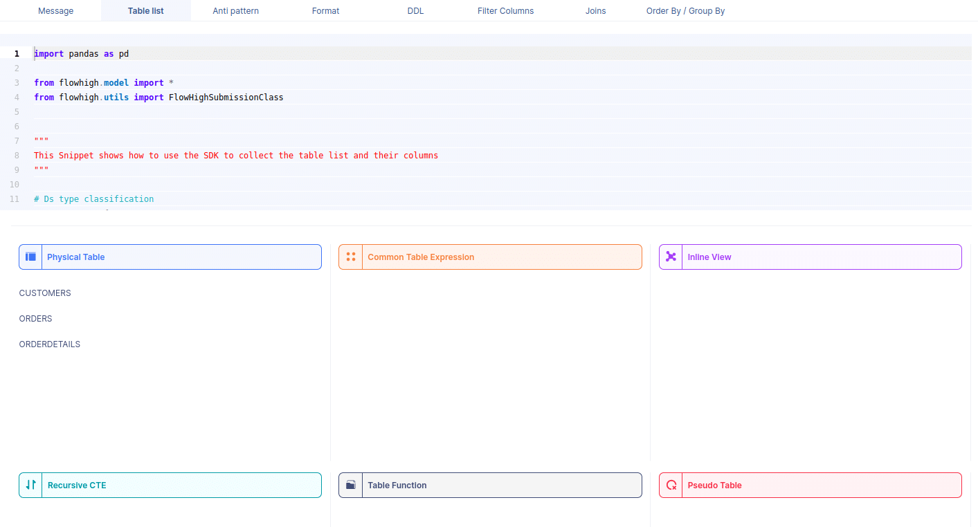
You can also access the FlowHigh SQL parser through the web based user interface. The below figure shows how FlowHigh provides the information about tables in a SQL query by grouping them into types of tables.

We took the Teradata SQL query example and parsed it through the web user interface.

We got the customer, orders and orderdetails tables back. As you can see the web UI also classifies these three tables as physical tables. Other types of tables are CTE, Views etc.

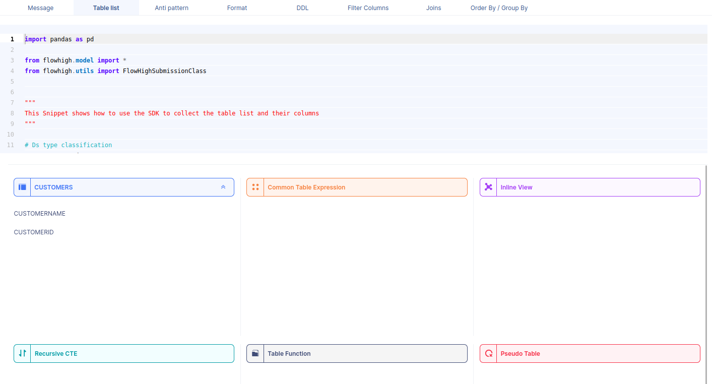
When we select a table name, it reveals the associated column names. For instance, by selecting the CUSTOMERS table, we can view its corresponding column names.

Likewise FlowHigh can be used to get columns used in a where conditions ,order by, group by and joins in the SQL query.

Columns used in GROUP BY / ORDER BY clause

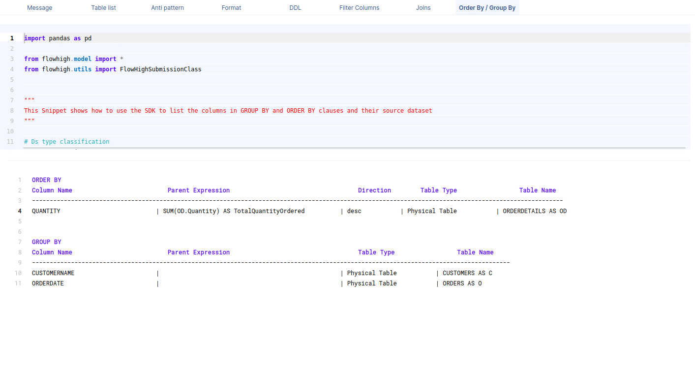
This figure shows how FlowHigh can be used to filter out the columns used in order by and group by clause.

Filter columns

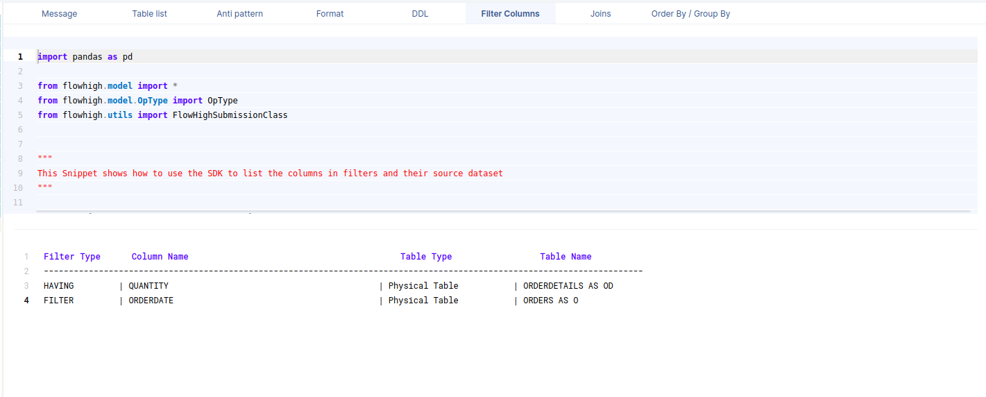
This figure shows how FlowHigh can be used to filter out the columns used in where clauses.

Columns in join conditions

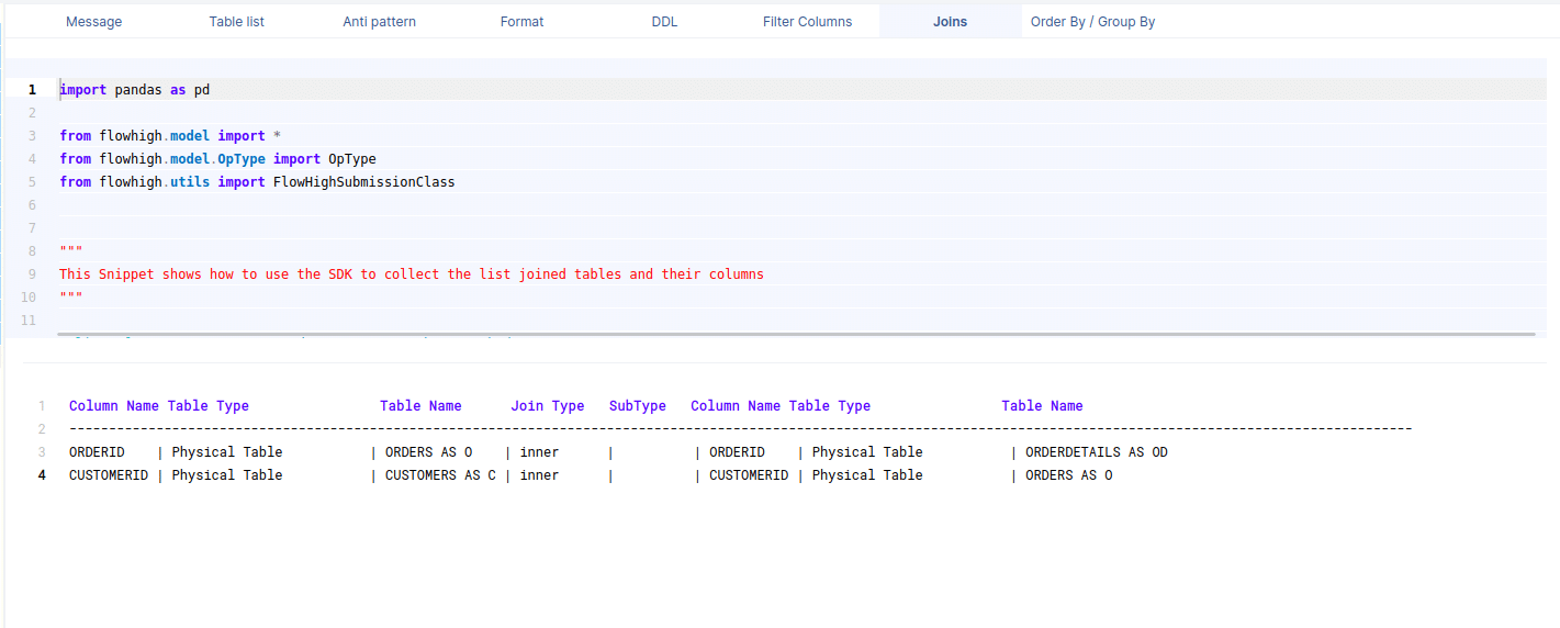
This figure shows how FlowHigh can be used to filter out the columns used and types of join. I have outlined in detail how this type of information can be very useful for data engineering scenarios to identify indexes, cluster keys etc.

Need more?

FlowHigh ships with two other modules

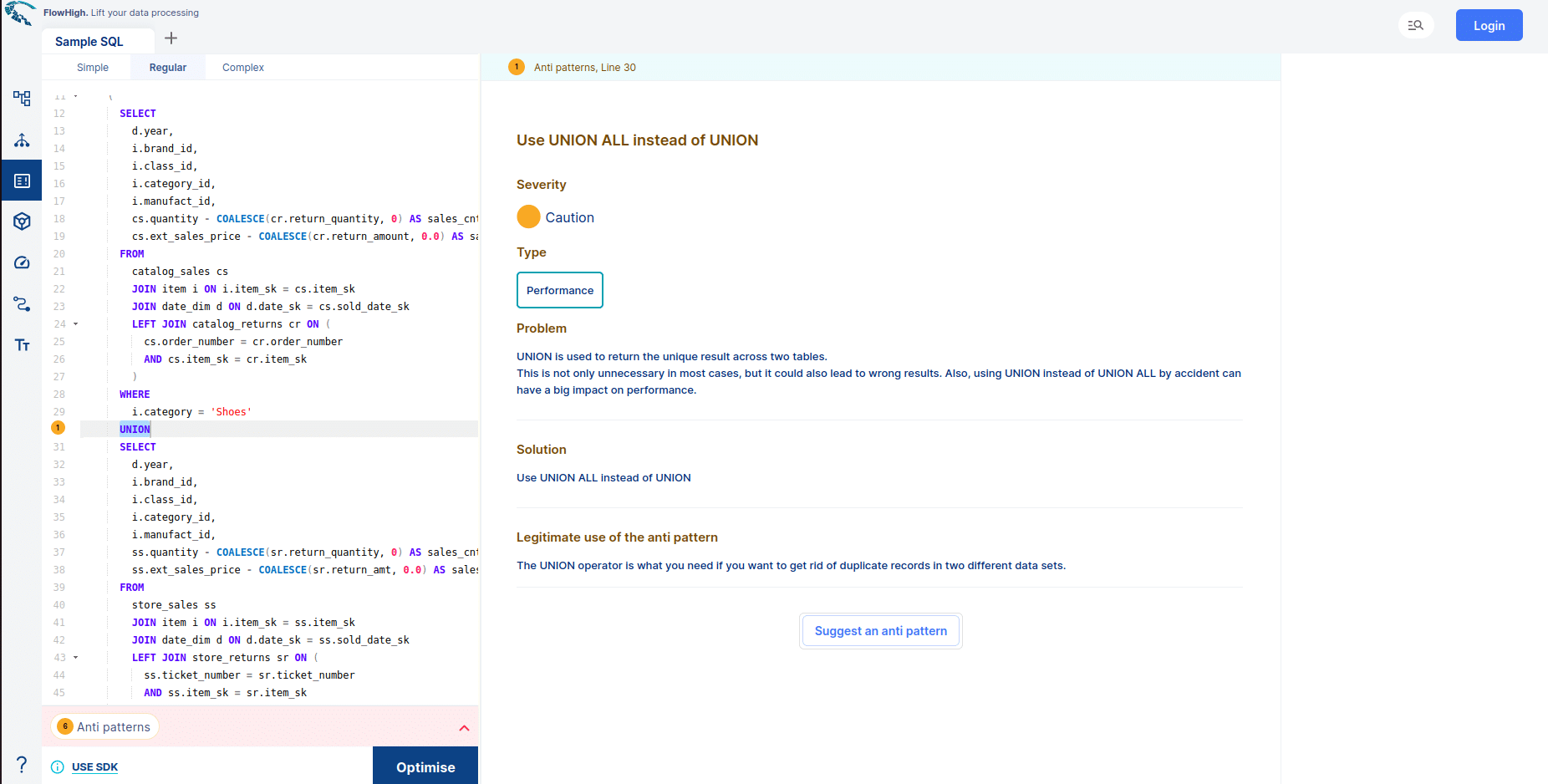
FlowHigh SQL Analyser. The Analyser checks for issues in your SQL coed. It detects 30+ anti patterns in SQL code

I have written up a blog post on automatically detecting bad SQL code.

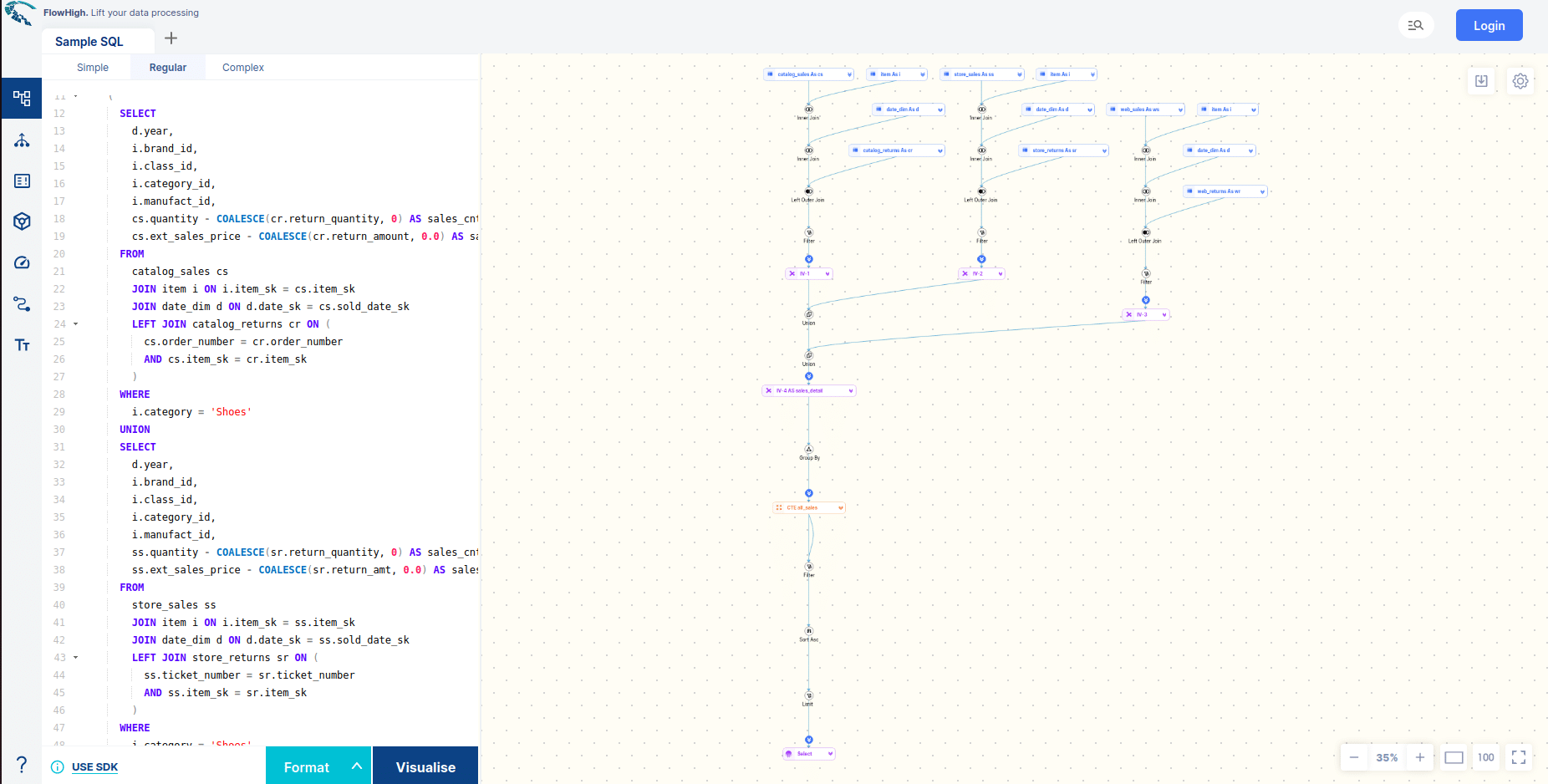
FlowHigh SQL Visualiser. Visualising SQL queries helps understand complex queries. It lets developers see how each part of the query contributes to the final result, making it easier to understand and debug.

You can try FlowHigh yourself. Register for the FlowHigh.

Back to Blog

Cookie	Duration	Description
__cfruid	session	Cloudflare sets this cookie to identify trusted web traffic.
cookielawinfo-checkbox-marketing	1 month	This cookie is set by the GDPR Cookie Consent plugin to store the user consent for the cookies in the category "Marketing".
cookielawinfo-checkbox-necessary	1 month	This cookie is set by GDPR Cookie Consent plugin. The cookies is used to store the user consent for the cookies in the category "Necessary".
cookielawinfo-checkbox-preferences	1 month	This cookie is set by the GDPR Cookie Consent plugin to check if the user has given consent to use cookies under the "Preferences" category.
cookielawinfo-checkbox-statistics	1 month	This cookie is set by the GDPR Cookie Consent plugin to store the user consent for the cookies in the category "Statistics".
cookielawinfo-checkbox-unclassified	1 month	This cookie is set by GDPR Cookie Consent plugin. The cookie is used to store the user consent for the cookies in the category "Unclassified".
CookieLawInfoConsent	1 month	Records the default button state of the corresponding category & the status of CCPA. It works only in coordination with the primary cookie.
csrftoken	1 year	This cookie is associated with Django web development platform for python. Used to help protect the website against Cross-Site Request Forgery attacks

Cookie	Duration	Description
AnalyticsSyncHistory	1 month	Linkedin set this cookie to store information about the time a sync took place with the lms_analytics cookie.
bcookie	2 years	LinkedIn sets this cookie from LinkedIn share buttons and ad tags to recognize browser ID.
bscookie	2 years	LinkedIn sets this cookie to store performed actions on the website.
lang	session	LinkedIn sets this cookie to remember a user's language setting.
li_gc	2 years	Linkedin set this cookie for storing visitor's consent regarding using cookies for non-essential purposes.
lidc	1 day	LinkedIn sets the lidc cookie to facilitate data center selection.
mgref	1 year	This cookie is set by Eventbrite to deliver content tailored to the end user's interests and improve content creation. It is also used for event-booking purposes.
mgrefby	1 year	This cookie is set by Eventbrite to deliver content tailored to the end user's interests and improve content creation. It is also used for event-booking purposes.
UserMatchHistory	1 month	LinkedIn sets this cookie for LinkedIn Ads ID syncing.

Cookie	Duration	Description
G	1 year	Cookie used to facilitate the translation into the preferred language of the visitor.
SERVERID	session	This cookie is set by Slideshare's HAProxy load balancer to assign the visitor to a specific server.

Cookie	Duration	Description
_ga	2 years	The _ga cookie, installed by Google Analytics, calculates visitor, session and campaign data and also keeps track of site usage for the site's analytics report. The cookie stores information anonymously and assigns a randomly generated number to recognize unique visitors.
_ga_7H38LVR4Z5	2 years	This cookie is installed by Google Analytics.
_gat_gtag_UA_44804396_1	1 minute	Set by Google to distinguish users.
_gat_UA-44804396-1	1 minute	A variation of the _gat cookie set by Google Analytics and Google Tag Manager to allow website owners to track visitor behaviour and measure site performance. The pattern element in the name contains the unique identity number of the account or website it relates to.
_gcl_au	3 months	Provided by Google Tag Manager to experiment advertisement efficiency of websites using their services.
_gid	1 day	Installed by Google Analytics, _gid cookie stores information on how visitors use a website, while also creating an analytics report of the website's performance. Some of the data that are collected include the number of visitors, their source, and the pages they visit anonymously.
CONSENT	2 years	YouTube sets this cookie via embedded youtube-videos and registers anonymous statistical data.
SIDCC	6 Months	The "SIDCC" cookie is used as security measure to protect users data from unauthorised access
test_cookie	15 minutes	The test_cookie is set by doubleclick.net and is used to determine if the user's browser supports cookies.
VISITOR_INFO1_LIVE	5 months 27 days	A cookie set by YouTube to measure bandwidth that determines whether the user gets the new or old player interface.
YSC	session	YSC cookie is set by Youtube and is used to track the views of embedded videos on Youtube pages.
yt-remote-connected-devices	never	YouTube sets this cookie to store the video preferences of the user using embedded YouTube video.
yt-remote-device-id	never	YouTube sets this cookie to store the video preferences of the user using embedded YouTube video.
yt.innertube::nextId	never	This cookie, set by YouTube, registers a unique ID to store data on what videos from YouTube the user has seen.
yt.innertube::requests	never	This cookie, set by YouTube, registers a unique ID to store data on what videos from YouTube the user has seen.

Cookie	Duration	Description
AN	1 month
AS	session
ebEventToTrack	1 month
eblang	1 year
SNID	2 years	This cookie is set by the Google. This cookie is used by the map which helps visitors to identify and reach the facility.
SP	session
SS	session

From Code to Clarity: Visualizing SQL code for Documentation and Debugging

From Code to Clarity: Visualizing SQL code for Documentation and Debugging

From Code to Clarity: Visualizing SQL code for Documentation and Debugging

From Code to Clarity: Visualizing SQL code for Documentation and Debugging

Deep dive on SQL parsing on Teradata

SQL parser for Teradata

Programmatically parsing the Teradata query history with the FlowHigh SDK

Analysing the output of the FlowHigh SQL parser

FlowHigh User Interface for SQL parsing

Deep dive on SQL parsing on Teradata

SQL parser for Teradata

Programmatically parsing the Teradata query history with the FlowHigh SDK

Analysing the output of the FlowHigh SQL parser

FlowHigh User Interface for SQL parsing

Related Articles

SQL Parsing for PostgreSQL Table and Column Audit Logging

Mastering SQL: How to detect and avoid 34+ Common SQL Antipatterns

AWS Athena SQL parser for table and column audit logging

Cookies consent