Data Exploration with Window Functions on Redshift
We have already introduced the main concept, syntax and simple examples of window functions applied to practical problems. In this post, we will go through some more advanced window functions and aim our focus on analytical use cases.
The dataset we will work with consists of information about phone calls and internet usage of two users. For each call, we know its duration in seconds and if the call was incoming or outgoing. In the latter case, we also know the phone number of the counterpart. We also have the information about the amount of data downloaded (measured in kB). Let’s see a sample:

Loading data from S3 to Redshift
The dataset is available through the following link: calls.tsv. The following code shows how to create a schema for our data and how to load the dataset from S3 storage to Redshift:
|
1 2 3 4 5 6 7 8 9 10 |
CREATE TABLE calls ( user_id INT NOTNULL ,date_time TIMESTAMP NOTNULL ,phone VARCHAR(256) NOTNULL ,duration INT ,data INT ); COPY calls FROM 's3://<bucket-name>/<path-to-calls.tsv>' IAM_ROLE 'arn:aws:iam::<aws-account-id>:role/<role-name>’ DELIMITER '\t' CSV IGNOREHEADER 1; |
MAX OVER() to identify Longest call
In the first exercise let’s print all calls together with the longest call that the user has ever made with the current counterpart. In addition, we would like to know the longest call in the current day to compare. Worth noting the important feature of the window functions: each OVER clause can use different aggregation independently. Let’s use aggregation over both the phone and date to demonstrate this feature. We will skip the incoming calls and internet usage.
|
1 2 3 4 5 6 7 8 9 10 11 12 |
SELECT user_id ,date_time ,phone ,(duration || ' secs') :: INTERVAL AS duration ,(MAX(duration) OVER ( PARTITION BY user_id, phone ) || ' secs') :: INTERVAL AS longest_for_number ,(MAX(duration) OVER ( PARTITION BY TRUNC(date_time) ) || ' secs') :: INTERVAL AS longest_today FROM calls WHERE phone != 'Internet' AND phone != 'incoming' ORDER BY user_id, date_time, phone; |
Output:
Rows with the same phone number are in the same colour. Notice that they share the same number_longest time. The duration time in bold marks the calls that were longest on a particular day. See the comparison with the longest_today column.
The aggregate function MAX together with the partitioning by phone clause computes the longest call made by a user and puts this against all user’s calls so we have this repeating extra column available for various comparisons. Using the traditional GROUP BY aggregation would require self-joining tables.
To extract a date from a timestamp, we use TRUNC function in the query. This expression is valid only for Redshift and equivalent in Postgres is DATE_TRUNC(‘day’, date_time). Also note that to convert the number of seconds in INT to INTERVAL, we concatenate the number with ‘ secs’string and then cast to INTERVAL with a double colon.
SUM function: Total duration over phone numbers
Let’s find out who receives the longest calls. In other words, we are interested in the total sum of call durations for the particular counterpart. Let’s also print the percentage of this sum relative to all user’s calls.
|
1 2 3 4 5 6 7 8 9 10 11 12 13 14 15 |
SELECT user_id ,date_time ,phone ,(SUM(duration) OVER ( PARTITION BY user_id, phone ) || ' secs') :: INTERVAL AS duration_by_phone ,SUM(duration) OVER ( PARTITION BY user_id, phone ) AS total_phone_secs ,CASE WHEN SUM(duration) OVER (PARTITION BY user_id) > 0 THEN round(100 * (SUM(duration) OVER ( PARTITION BY user_id, phone ) / (SUM(duration) OVER (PARTITION BY user_id)))) ELSE 0 END AS percentage FROM calls WHERE phone != 'Internet' AND phone != 'incoming' ORDER BY date_time; |
Let’s understand the query starting from the inner core section:
- The total duration over user and phone is computed by the window function SUM and partitioned by the mentioned fields. The same is applied to INTERVAL and INT type.
- To compute the percentage, we use the previously mentioned expression in the numerator and sum over all calls in the denominator. The type of duration is INT, which would cause the division to give integer result, and therefore we need to cast the denominator to FLOAT before the division. After the division, the result is multiplied by 100 and rounded to get the percentage.
- The CASE clause checks if the total duration is greater than 0 so that we do not divide by zero. If the condition is false, there are only calls of zero length for the phone number, hence we return 0 as the total duration in this case.
- The WHERE clause collects only rows with outgoing calls since we do not know the phone number of incoming calls.
Window functions produce an output row for each call, but similar to the previous example all rows with the same phone number contain the same aggregated information.
Output:
We can discover from the percentage column for example, that the first user spent almost half of his calling time by calling number 49508432274. Some other numbers took less than 1 percent of total call time.
Lead function: Periods of inactivity
Anytime we need to calculate values based on neighbouring rows, window functions should be the first thing that come to mind. A good example for our dataset would be periods of inactivity between calls. Let’s say we want to see all periods of inactivity longer than 2 days for each user. We will consider internet usage as an instant activity with no duration and calls as an activity with the specified duration. This scenario is also very useful for identification and segmentation of sessions in a clickstream data, also known as sessionization.
To get starts and ends of the periods, we will take advantage of the LEAD function, which behaves as the LAG function, however, instead of the previous rows, it looks up the following ones.
|
1 2 3 4 5 6 7 8 9 10 11 12 |
SELECT * FROM (SELECT user_id ,date_time + (COALESCE(duration, 0) || ' secs') :: INTERVAL AS period_from ,LEAD(date_time) OVER ( PARTITION BY user_id ORDER BY date_time ) AS period_to ,LEAD(date_time) OVER ( PARTITION BY user_id ORDER BY date_time ) - (date_time + (COALESCE(duration, 0) || ' secs'):: INTERVAL) AS duration ,EXTRACT(EPOCH FROM LEAD(date_time) OVER ( PARTITION BY user_id ORDER BY date_time ) - date_time) - COALESCE(duration, 0) AS duration_in_secs FROM calls ) AS periods WHERE duration > '2 days' ORDER BY user_id, period_from; |
The beginning of a period is computed as a sum of the starting date, time and duration of the call. The COALESCE function ensures that for the internet usage, the duration is zero since the function returns 0 anytime duration field is null. Period of inactivity ends when the following activity begins, therefore LEAD function extracts time of the next activity in the sequence ordered by date and time partitioned by a user. The next two columns are just differences of the first two columns in INT and INTERVAL type.
The outer SELECT puts a threshold on the period length and filters only periods longer than 2 days. The following table shows the output of the query. Notice the last periods for each user – both of them did not use the phone for more than a week.
Ntile function: Producing Quartiles
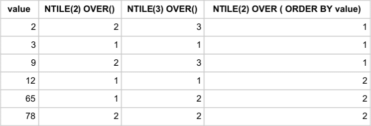
If a dataset becomes large enough, we could be interested in some statistical measures. The window function NTILE(num_buckets) enables us to compute quantiles. It divides the partition as equally as possible by assigning numbers 1..num_buckets to rows. Let’s see an example for the following new dataset of six values: [12,3,65,78,2,9]
The second and third column show how NTILE function assigns numbers to all values so that each bucket has an equal number of rows. In the second column, clause NTILE(2) ensures that the values are divided into two buckets, represented by numbers 1 and 2. The same principle is applied in the third column but now with three buckets and numbers 1,2,3. The buckets are, however, unrelated to the values itself and the assignment is basically random. The last column specifies ORDER BY clause, which forces the function to number ordered sequence of values. Therefore, lower numbers are assigned to the lower values.
When the ORDER BY clause is specified, we can interpret the output as division into quantiles taking data as the split criteria. In the case of internet usage, the task is to find quartiles of the data usage distribution. Let’s see the result of the NTILE function together with ordering by data.
Code:
|
1 2 3 4 5 6 7 |
SELECT date_time ,data ,NTILE(4) OVER ( ORDER BY data ) AS quartile FROM calls WHERE phone = 'Internet' ORDER BY data; |
Output:
Neither the date nor time is important now, but we can see that the rows are ordered by data_usage, and therefore, the quartiles can be computed as follows:
|
1 2 3 4 5 6 7 8 9 10 11 12 |
SELECT quartile ,MIN(data) AS from ,MAX(data) AS to FROM (SELECT date_time ,data ,NTILE(4) OVER ( ORDER BY data ) AS quartile FROM calls WHERE phone = 'Internet') AS quartiles GROUP BY quartile ORDER BY quartile; |
Using aggregate functions MIN and MAX we compute the range of the quartile intervals.
Besides quartiles, we can derive the median from the output as (1303 + 1321) / 2 = 1312. Worth noting the alternative, simpler way to compute median by using percentile_cont(fraction) function together with clause
WITHIN GROUP:
|
1 2 3 4 |
SELECT percentile_cont(0.5) WITHIN GROUP (ORDER BY data) FROM calls WHERE phone = 'Internet'; |
This code gives us median 1301.5, so which one is correct? The percentile_cont computes the correct median, but what went wrong with the first approach? The answer lies behind the algorithm of NTILE function. Let’s see the result of the NTILE function with 2 buckets instead of 4:
Now the median truly follows (1300 + 1303) / 2 = 1301.5. For a better understanding, we will print counts of the rows assigned to quartiles by NTILE function.
We can see that whenever it is not possible to make buckets of equal size, the NTILE function assigns more rows to the top buckets. That is why the first two groups contain 934 rows, whereas the other two groups contain only 932. Then the median is incorrectly computed from values shifted by one row. Of course, when the number of buckets is 2, both the groups contain 933 rows.
Redshift has an even simpler syntax for computing median since MEDIAN is one of the window functions.
|
1 2 3 4 5 |
SELECT MEDIAN(data) OVER () AS median FROM calls WHERE phone = 'Internet' LIMIT 1; |
Note that we limit the output to one line only because window functions always return a result for all rows, which would create unnecessary duplicates. Oracle supports the MEDIAN function as well but for example, PostgreSQL does not.